

It is well-known that you can use the RF Module to compute the impedance of lossless transmission line structures, such as coaxial cables of uniform cross section. But did you know that you can also compute an effective impedance for waveguides with non-uniform cross section? Let’s find out how!
Computing the Impedance of a Straight Coaxial Cable
First, let’s look at one of the most common transmission line structures, the coaxial cable. An inner and outer conductor are separated by a dielectric, and a wave will travel along the length of the cable in a TEM mode, meaning that the electric and magnetic field are transverse to the direction of propagation.
If we can assume that the conductors and the dielectric are lossless (a good approximation for many cases), we can compute an impedance, as demonstrated in the Model Gallery benchmark example on Finding the Impedance of a Coaxial Cable (the model can also be found in the Model Library).
In that example, we draw a 2D cross section of the coax and specify the dielectric properties as well as an operating frequency below the cutoff frequency for any TE or TM modes. The COMSOL software will then solve an eigenvalue problem for the out-of-plane propagation constant as well as the fields, which can be used to compute the impedance of the cable. This approach is very efficient in terms of computation, but only works for TEM waveguides of uniform cross section.
Computing the Impedance of a Corrugated Coaxial Cable
Now, let’s consider a coaxial waveguide with a corrugated outer conductor. These are used when mechanical flexibility is desired.
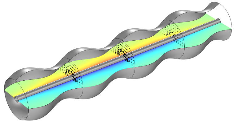
A corrugated coaxial cable. The slice plot is of the electric field and the arrow plot is the magnetic field.
Such waveguides will not be operating in a purely TEM mode, meaning that there is some electric and magnetic field component in the direction of propagation. However, we will assume that these components are small and can, as a consequence, define the impedance as:
where V is the voltage that can be evaluated by taking the path integral of the electric field at any line between the inner and outer conductor, and P is the integral of the Poynting flux at any cross section. You can use Integration Coupling Operators to evaluate the fields at the edges and boundaries of the modeling domain to evaluate these quantities.
Defining a Unit Cell Model
Rather than computing a long section of the waveguide, we can consider only one periodic section of the structure itself. But the effective wavelength of the signal traveling down the waveguide will be much longer than this, so we use the Floquet periodic boundary condition to specify that the wave traveling down the waveguide has a specified propagation constant.
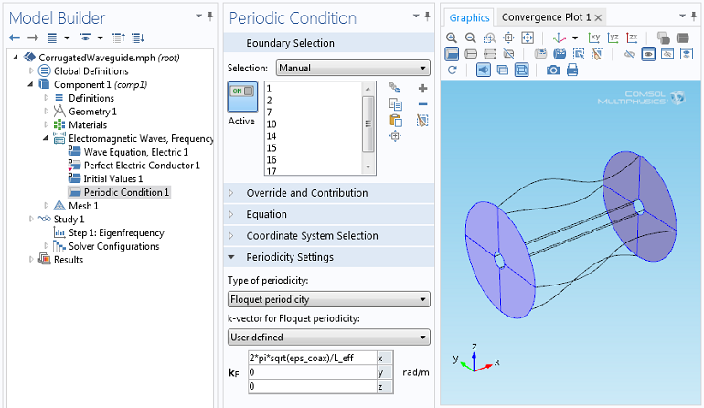
The Floquet periodic boundary condition interface.
Via this approach, we can then solve an eigenvalue problem to compute the frequency of the wave that will have this propagation constant. When using a periodic boundary condition, we also need to ensure that the mesh on the boundaries is periodic.
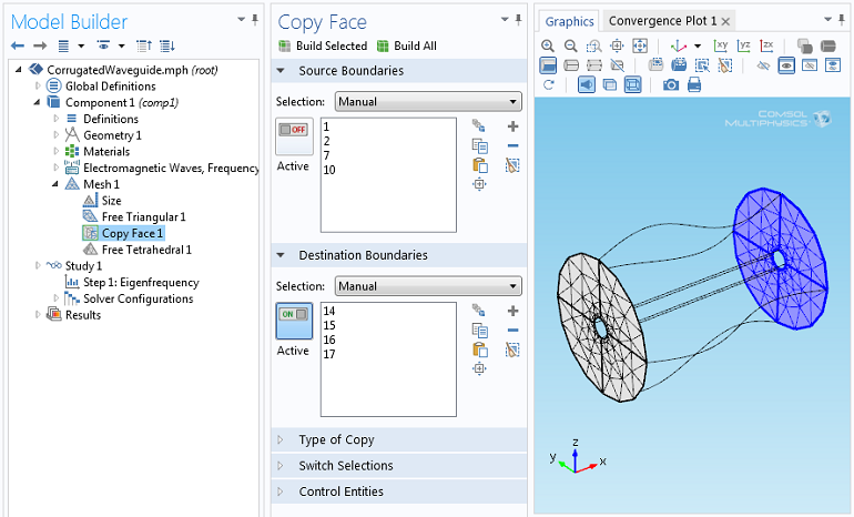
The Copy Face feature will ensure that the mesh on the periodic faces is identical. The interior is then meshed with free tetrahedral elements.
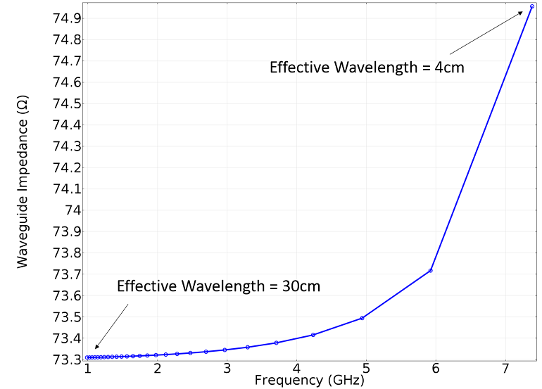
Once the solution is computed for a single unit cell, we can evaluate the impedance at that frequency. We can also sweep over a range of effective wavelengths to compute the impedance over a range and observe that at higher frequencies, the impedance will go up. This means that we are approaching the frequency at which TE or TM modes will be present. At that point, we can no longer use this approach.
Concluding Remarks
Here, we have shown that you can compute an impedance for a waveguide with periodic structure operating in the quasi-TEM regime. The Floquet Periodic boundary conditions and the Copy Face functionality are used to set up a unit cell model, which is solved to extract the impedance for a range of frequencies.
If you have questions about this type of modeling, please contact us.


Comments (2)
Zhijie Ma
May 23, 2016Hi, Walter, is it possible that you can share the model file? Thank you.
Bridget Cunningham
May 23, 2016Hi Zhijie,
Thank you for your question.
Please contact our support team.
Online support center: https://www.comsol.com/support
Email: support@comsol.com
Best,
Bridget