

This post continues our blog series on the weak formulation. In the previous post, we implemented and solved an exemplary weak form equation in the COMSOL Multiphysics software. The result was validated with simple physical arguments. Today, we will start to take a behind-the-scenes look at how the equations are discretized and solved numerically.
Our Simple Example
Recall our simple example of 1D heat transfer at steady state with no heat source, where the temperature T is a function of the position x in the domain defined by the interval 1\le x\le 5. With the boundary conditions that the outgoing flux should be 2 at the left boundary (x=1) and the temperature should be 9 at the right boundary (x=5), the weak form equation reads:
(1)
We now attempt to find a way to solve this equation numerically.
Basis Functions
To solve Eq. (1) numerically, we first divide the domain 1\le x\le 5 into four evenly spaced sub-intervals, or mesh elements, bound by five nodal points x = 1, 2, \cdots, 5. Then, we can define a set of basis functions, or shape functions, \psi_{1L}(x), \psi_{1R}(x), \psi_{2L}(x), \psi_{2R}(x), \cdots, \psi_{4R}(x), as shown in the graph below, where there are two shape functions in each mesh element, represented by a solid line and a dashed line.
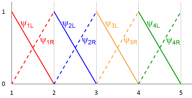
For example, in the first element (1 \le x \le 2), we have
(2)
\psi_{1L}(x) %26=%26 \left\{ \begin{array}{ll}
2-x \mbox{ for } 1 \le x \le 2,\\
0 \mbox{ elsewhere}
\end{array} \right \mbox{ (solid red line)}
\end{equation}
\psi_{1R}(x) %26=%26 \left\{ \begin{array}{ll}
x-1 \mbox{ for } 1 \le x \le 2, \\
0 \mbox{ elsewhere}
\end{array} \right \mbox{ (dashed red line)}
\end{equation}
We observe that each shape function is a simple linear function ranging from 0 to 1 within a mesh element, and vanishes outside of that mesh element.
Note: Of course, COMSOL Multiphysics allows shape functions formed with higher-order polynomials, not just linear functions. The choice of linear shape functions here is for visual clarity.
With this set of shape functions, we can approximate any arbitrary function defined in the domain 1\le x\le 5 by a simple linear combination of them:
(3)
where a_{1L}, a_{1R}, a_{2L}, a_{2R}, \cdots are some constant coefficients, one for each shape function. In the graph below, the arbitrary function u(x) is represented by the black curve. The cyan curve represents the approximation by the superposition of the shape functions (3). Each term on the right-hand side of Eq. (3) is plotted using the same color and line style as the graph above.
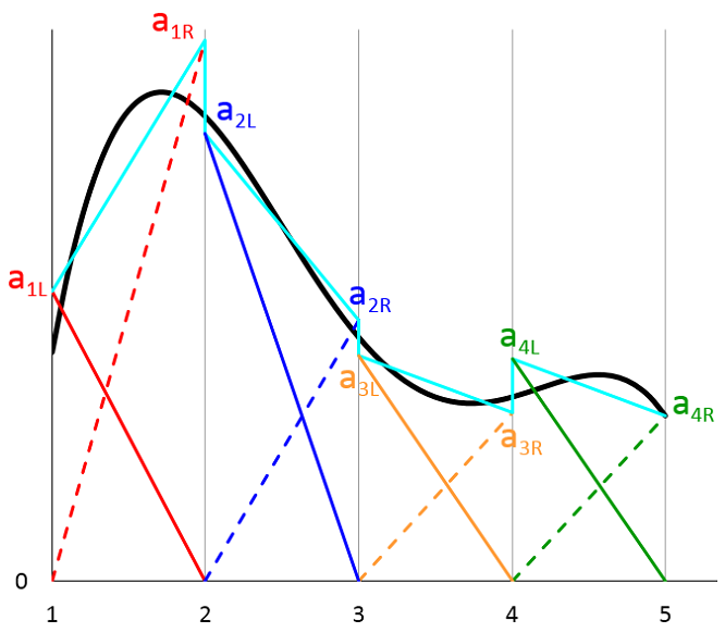
We see that in general the approximation (represented by the cyan curve) can be discontinuous across the boundary between adjacent mesh elements. In practice, many physical systems, including our simple example of heat conduction, are expected to have continuous solutions. For this reason, the default shape functions for most physics interfaces are Lagrange elements, in which the shape function coefficients are constrained so that the solution is continuous across boundaries between adjacent elements. In this case, the approximation is simplified, as shown in the figure below,
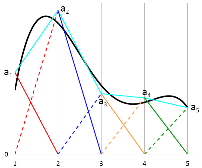
where the cyan curve has been made continuous by setting the coefficients on each side of a mesh boundary to be equal: a_{1R} = a_{2L}, a_{2R} = a_{3L}, a_{3R} = a_{4L}. We also renamed the coefficients for brevity:
\begin{align}
a_1 %26\equiv a_{1L}\\
a_2 %26\equiv a_{1R} = a_{2L}\\
a_3 %26\equiv a_{2R} = a_{3L}\\
a_4 %26\equiv a_{3R} = a_{4L}\\
a_5 %26\equiv a_{4R}
\end{align}
\end{equation*}
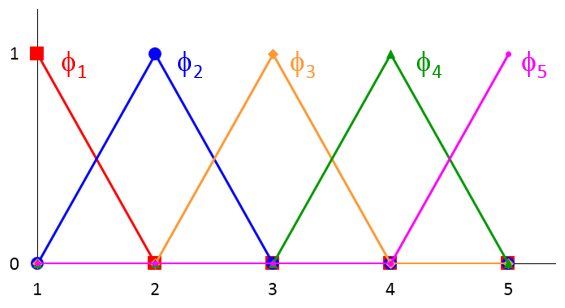
We see that the continuity condition requires pairs of shape functions to share the same coefficient in making the approximation (3), which can now in turn be simplified by combining those pairs of shape functions into a new set of basis functions ϕ1(x),ϕ2(x),⋯,ϕ5(x), with each function localized around a nodal point:
(4)
\begin{align}
\phi_1(x) \equiv \psi_{1L}(x) %26= \left\{ \begin{array}{ll}
2-x \mbox{ for } 1\:$\leq$\:\textit{x}\:$\leq$\:2,\\
0 \mbox{ elsewhere}
\end{array} \right
\\
\phi_2(x) \equiv \psi_{1R}(x) + \psi_{2L}(x) %26= \left\{ \begin{array}{lll}
x-1 \mbox{ for } 1\:$\leq$\:\textit{x}\:$\leq$\:2, \\
3-x \mbox{ for } 2\:\textless\:x\:$\leq$\:3, \\
0 \mbox{ elsewhere}
\end{array} \right
\\
\phi_3(x) \equiv \psi_{2R}(x) + \psi_{3L}(x) %26= \left\{ \begin{array}{lll}
x-2 \mbox{ for } 2\:$\leq$\:\textit{x}\:$\leq$\:3, \\
4-x \mbox{ for } 3\:\textless\:x\:$\leq$\:4, \\
0 \mbox{ elsewhere}
\end{array} \right
\\
\\ \cdot
\\ \cdot
\\ \cdot
\end{equation*}
As shown in the graph below, each new basis function is essentially a triangular-shaped, piecewise-linear function centered around a nodal point. Its value varies between 1 and 0 within the mesh element(s) adjacent to the nodal point, and vanishes everywhere else.
As discussed above, by choosing this new set of basis functions, we constrain the solution to be continuous across the boundary between adjacent mesh elements. Most physical systems satisfy this continuity constraint, including our simple heat transfer example here.
Now, with this new set of basis functions, the approximation (3) is simplified to
(5)
In the graph below, the arbitrary function u(x) is represented by the black curve. The cyan curve represents the approximation by the superposition of the new basis functions. Each term on the right-hand side of Eq. (5) is plotted using the same color scheme as the graph above.
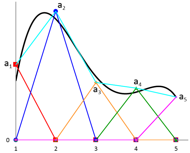
As an aside, if the black curve represents the exact solution to some real modeling problem, then we see that the approximation is not very good, due to the coarseness of the mesh. Also, in general, the nodal point values a_1, a_2, \cdots are not required to lie on the exact solution, unless one is constrained to a known solution value (shown in a_5 as an example in the figure above). The discrepancy between the black and the cyan curves we see here represents the discretization error of the solution. In 2D and 3D models, there will also be a discretization error of the geometry. In my colleague Walter Frei’s blog post on meshing considerations, both types of errors are discussed in some detail. Due to these potential errors, a mesh refinement study is necessary to ensure the accuracy of modeling results.
We note that the approximation given by Eq. (5) (the cyan curve) is piecewise-linear. Thus, it’s impossible to evaluate its second derivatives numerically. As we have mentioned before, the weak formulation provides numerical benefits by reducing the order of differentiation in the equation system. In this case, only the first derivative is needed and it can be readily evaluated numerically. In a future blog entry, we will discuss an example of discontinuity in the material property that also benefits from the reduced order of differentiation.
Discretizing the Weak Form Equation in Two Steps
With the new set of basis functions defined above, we proceed to discretize the weak form equation (1) in two steps. First, the temperature function, T(x), can be approximated by the set of basis functions in the same way as in Eq. (5):
(6)
where a_1, a_2, \cdots , a_5 are unknown coefficients to be determined.
Substituting the expression for T(x) (6) into the weak form equation (1), we obtain
(7)
a_1 \int_1^5 \partial_x \phi_1(x) \partial_x \tilde{T}(x) \,dx + a_2 \int_1^5 \partial_x \phi_2(x) \partial_x \tilde{T}(x) \,dx + \cdots + a_5 \int_1^5 \partial_x \phi_5(x) \partial_x \tilde{T}(x) \,dx
\\
= -2 \tilde{T}_1 -\lambda_2 \tilde{T}_2 -\tilde{\lambda}_2 (a_5 -9)
\end{array}
where the temperature at the right boundary x=5, T_2, has been evaluated using the expression (6) and the fact that the basis functions are localized, leading to only one term, a_5 \phi_5(x=5) = a_5, contributing to T(x=5).
We see that there are six unknowns in the discretized version of the weak form equation (7): The five coefficients a_1, a_2, \cdots , a_5 and the one flux \lambda_2 at the right boundary. It is customary to call the unknowns degrees of freedom. For example, here we say the (discretized) problem has “six degrees of freedom”.
To solve for the six unknowns, we need six equations. This leads to the second step of discretization. Recall from our first blog post that the role of the test functions is to sample the equation locally to clamp down the solution everywhere within the domain. Now we already have a set of localized functions, our basis functions \phi_1, \cdots, \phi_5, so we can just substitute them into the test function \tilde{T} in Eq. (7) to obtain the six equations we need.
Here is a table showing the six substitutions that will generate the six equations for us:
| \tilde{T}(x) | \tilde{\lambda}_2 |
|---|---|
| \phi_1(x) | 0 |
| \phi_2(x) | 0 |
| \phi_3(x) | 0 |
| \phi_4(x) | 0 |
| \phi_5(x) | 0 |
| 0 | 1 |
Since each of the basis functions is localized, each substitution yields an equation with a small number of terms. For example, the first substitution gives
a_1 \int_1^5 \partial_x \phi_1(x) \partial_x \phi_1(x) \,dx + a_2 \int_1^5 \partial_x \phi_2(x) \partial_x \phi_1(x) \,dx + \cdots + a_5 \int_1^5 \partial_x \phi_5(x) \partial_x \phi_1(x) \,dx
\\
= -2 \phi_1(x=1) -\lambda_2 \phi_1(x=5) -0 (a_5 -9)
\end{array}
We note that \phi_1 has non-trivial overlap only with itself and \phi_2. Therefore, only the first two terms on the left-hand side are non-zero. Also, \phi_1 is localized near the left boundary (x=1), so only the first term on the right-hand side remains. The equation now becomes
(8)
where we have evaluated the definite integrals on the left-hand side:
\begin{align}
\int_1^5 \partial_x \phi_1(x) \partial_x \phi_1(x) \,dx %26= 1\\
\int_1^5 \partial_x \phi_2(x) \partial_x \phi_1(x) \,dx %26= -1\\
\end{align}
\end{equation*}
and used the definition of \phi_1 on the right-hand side: \phi_1(x=1) = 1.
Similarly, the remaining five substitutions listed in the table above yield these equations:
(9)
\begin{align}
-a_1 + 2 a_2 -a_3 %26= 0\\
-a_2 + 2 a_3 -a_4 %26= 0\\
-a_3 + 2 a_4 -a_5 %26= 0\\
-a_4 + a_5 %26= -\lambda_2\\
0 %26= -(a_5 -9)\\
\end{align}
\end{equation*}
We now have six equations for our six unknowns and it is straightforward to verify that the solution matches what we have obtained using COMSOL Multiphysics software in the previous post. For example, the last equation immediately gives us a_5 = 9, and using the expression (6) for the temperature, we obtain its value at the right boundary:
\begin{align}
T(x=5) %26= a_1 \phi_1(x=5) + a_2 \phi_2(x=5) + \cdots + a_5 \phi_5(x=5)\\
%26= a_1 \cdot 0 + a_2 \cdot 0 + \cdots + a_5 \cdot 1\\
%26= 9\\
\begin{align}
\end{equation*}
This agrees with the fixed boundary condition that the temperature should be 9 at the right boundary. It is also easy to see that it is the term associated with the test function \tilde{\lambda}_2 that gives rise to the equation (0 = a_5 -9), as we would expect.
Matrix Representation
It is convenient to write the discretized system of equations (in our simple example, there are six equations given in (8) and (9)) in terms of matrices and vectors:
(10)
\begin{array}{cccccc}
1 & -1 & 0 & 0 & 0 & 0 \\
-1 & 2 & -1 & 0 & 0 & 0 \\
0 & -1 & 2 & -1 & 0 & 0 \\
0 & 0 & -1 & 2 & -1 & 0 \\
0 & 0 & 0 & -1 & 1 & 1 \\
0 & 0 & 0 & 0 & 1 & 0
\end{array}
\right)
\left(
\begin{array}{c} a_1 \\ a_2 \\ a_3 \\ a_4 \\ a_5 \\ \lambda_2 \end{array}
\right)
= \left(
\begin{array}{c} -2 \\ 0 \\ 0 \\ 0 \\ 0 \\ 9 \end{array}
\right)
The matrix on the left-hand side is customarily called the stiffness matrix and the vector on the right is called the load vector, due to the application of this technique in structural mechanics.
We notice two interesting facts about this matrix equation. First, there are a lot of zeros in the matrix (a so-called sparse matrix). In a practical model where there are many more mesh elements than our four elements here, we can envision that most of the elements in the matrix will be zero. This is a direct benefit of choosing localized shape functions, and it lends itself to very efficient numerical methods to solve the equation system.
Second, the Lagrange multiplier \lambda_2 appears only in one equation (the last column of the matrix has only one non-zero element). The remaining five equations involve only the five unknown coefficients a_1, a_2, \cdots , a_5. Therefore, we can choose to solve for a_1, a_2, \cdots , a_5 using the five equations, without ever needing to solve for \lambda_2. As we briefly mentioned in the previous entry, in general, it is possible to choose not to solve for the Lagrange multiplier(s) in order to gain computation speed.
Summary and Next Topic in the Weak Form Series
Today, we reviewed the basic procedure for discretizing the weak form equation using our simple example. We took advantage of a set of localized shape functions in two steps:
- Using them as a basis to approximate the real solution
- Substituting them one by one into the weak form equation to obtain the discretized system of equations
The resulting matrix equation is sparse, which can be solved efficiently using a computer.
In the previous blog post, when we implemented the weak form equation using COMSOL Multiphysics, the discretization was done under the hood without needing the user’s help. Next, we will show you how to inspect the stiffness matrix and load vector, as well as how to choose to solve for — or not to solve for — the Lagrange multiplier by using the Weak Form PDE interface in the software.

Comments (7)
Priyanka Agrawal
February 23, 2017Nice article 🙂
Yu Zhang
January 14, 2019Hi, Dr. Liu:
Thank you for sharing us this nice article. I encounter a problem when trying to discretize a weak form I developed by myself. However, in the weak form, there is a integration of the independent variable over an element volume (rather than over the whole geometry), like: (f p dVe)/Ve, f here denotes the integration symbol. This is actually a stabilized term I introduced to avoid pressure oscillations. Could you please share me some idea about how to deal with this term in weak form.
Thank you so much for your help and time.
Brianne Costa
January 15, 2019Hello Yu,
Thank you for your comment.
For questions related to your modeling, please contact our Support team.
Online Support Center: https://www.comsol.com/support
Email: support@comsol.com
Le Wen-Kai
May 24, 2019Dear Dr. Liu
Thank you for your sharing, but the equation (4) can’t be seen in the article.
Brianne Christopher
May 24, 2019Hi Le,
Please perform a hard refresh of your browser and you should be able to view equation 4.
Thank you,
Brianne
Le Wen-Kai
May 31, 2019No problem for visiting now, and thank you for your update!
Space lab
July 27, 2023Hi, Dr. Liu:
If the PDE is of third order, should we reduce it until we end up with terms involving first order derivative terms. or is it enough to get an equation involving second order terms after applying integration by parts.