

Electrochemical impedance spectroscopy is a versatile experimental technique that provides information about an electrochemical cell’s different physical and chemical phenomena. By modeling the physical processes involved, we can constructively interpret the experiment’s results and assess the magnitudes of the physical quantities controlling the cell. We can then turn this model into an app, making electrochemical modeling accessible to more researchers and engineers. Here, we will look at three different ways of analyzing EIS: experiment, model, and simulation app.
Electrochemical Impedance Spectroscopy: The Experiment
Electrochemical impedance spectroscopy (EIS) is a widely used experimental method in electrochemistry, with applications such as electrochemical sensing and the study of batteries and fuel cells. This technique works by first polarizing the cell at a fixed voltage and then applying a small additional voltage (or occasionally, a current) to perturb the system. The perturbing input oscillates harmonically in time to create an alternating current, as shown in the figure below.
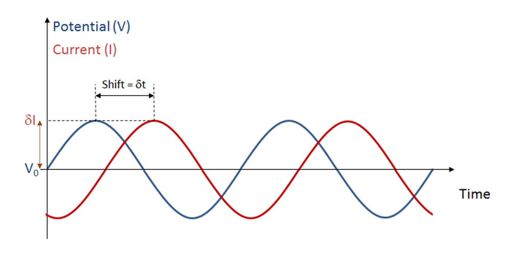
An oscillating perturbation in cell voltage gives an oscillating current response.
For a certain amplitude and frequency of applied voltage, the electrochemical cell responds with a particular amplitude of alternating current at the same frequency. In real systems, the response may be complicated for components of other frequencies too — we’ll return to this point below.
EIS experiments typically vary the frequency of the applied perturbation across a range of mHz and kHz. The relative amplitude of the response and time shift (or phase shift) between the input and output signals change with the applied frequency.
These factors depend on the rates at which physical processes in the electrochemical cell respond to the oscillating stimulus. Different frequencies are able to separate different processes that have different timescales. At lower frequencies, there is time for diffusion or slow electrochemical reactions to proceed in response to the alternating polarization of the cell. At higher frequencies, the applied field changes direction faster than the chemistry responds, so the response is dominated by capacitance from the charge and discharge of the double layer.
The time-domain response is not the simplest or most succinct way to interpret these frequency-dependent amplitudes and phase shifts. Instead, we define a quantity called an impedance. Like resistance in a static system, impedance is the ratio of voltage to current. However, it uses the real and imaginary parts of a complex number to represent the relation of both amplitude and phase to the input signal and output response. The mathematical tool that relates the impedance to the time-domain response is a Fourier transform, which represents the frequency components of the oscillating signal.
To explain the idea of impedance more fully for a simple case, consider the input voltage as a cosine wave oscillating at an angular frequency (ω):
Then the response is also a cosine wave, but with a phase offset (φ). Compared to the time shift in the image above, the phase offset is given as \phi = -\omega \,\delta t . The magnitude of the current and its phase offset depend on the physics and chemistry in the cell.
Now, let’s consider the resistance from Ohm’s law:
This quantity varies in time with the same frequency as the perturbing signal. It equals zero at times when the numerator also equals zero and becomes singular when the denominator equals zero. So unlike the resistance in a DC system, it’s not a very useful quantity!
Instead, from Euler’s theorem, let’s express the time-varying quantities as the real parts of complex exponentials, so that:
and
We denote the coefficients V_0 and I_0\,\exp(i\phi) as quantities \bar{V} and \bar{I}, respectively.
These are complex amplitudes that can be understood in terms of the Fourier transformation of the original time-domain sinusoidal signals. They express the distinct amplitudes and phase difference of the voltage and current. Because all of the quantities in the system are oscillating sinusoidally, we understand the physical effects by comparing these complex quantities, rather than the time-domain quantities. To describe the oscillating problem (often called phasor theory), we define a complex analogue of resistance as:
This is the impedance of the system and, as the name suggests, it’s the quantity we measure in electrochemical impedance spectroscopy. It’s a complex quantity with a magnitude and phase, representing both resistive and capacitive effects. Resistance contributes the real part of the complex impedance, which is in-phase with the applied voltage, while capacitance contributes the imaginary part of the complex impedance, which is precisely out-of-phase with the applied voltage.
EIS specialists look at the impedance in the form of a spectrum, normally with a Nyquist plot. This plots the imaginary component of impedance against the real component, with one data point for every frequency at which the impedance has been measured. Below is an example from a simulation — we’ll discuss how it’s modeled in the next section.
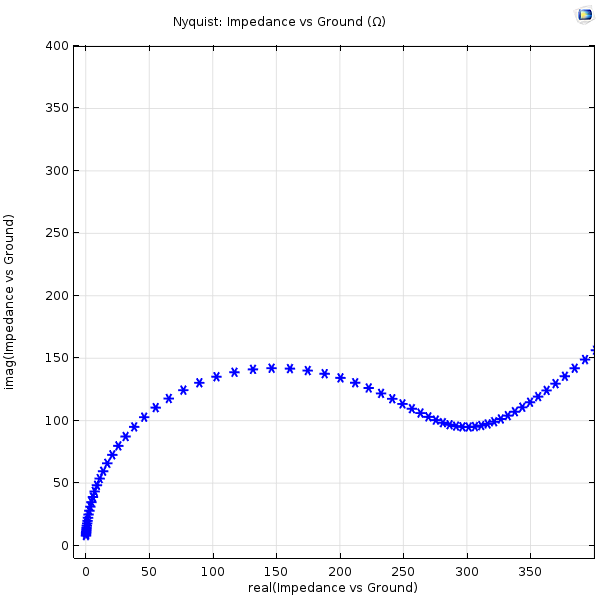
Simulated Nyquist plot from an electrochemical impedance spectroscopy experiment. Points toward the top right are at lower frequencies (mHz), while those toward the bottom left are at higher frequencies (>100 Hz).
In the figure above, the semicircular region toward the left side shows the coupling between double-layer capacitance and electrode kinetic effects at frequencies faster than the physical process of diffusion. The diagonal “diffusive tail” on the right comes from diffusion effects observed at lower frequencies.
EIS experiments are useful because information about many different physical effects can be extracted from a single analysis. There is a quantitative relationship between properties like diffusion coefficients, kinetic rate constants, and dimensions of the features in Nyquist plots. Often, EIS experiments are interpreted using an “equivalent circuit” of resistors and capacitors that yields a similar frequency-dependent impedance to the one shown in the Nyquist plot above. This idea was discussed in my colleague Scott’s blog post on electrochemical resistances and capacitances.
When there is a linear relation between the voltage and current, only one frequency will appear in the Fourier transform. This simplifies the analysis significantly.
For the simple harmonic interpretation of the experiment in terms of impedance, we need the current response to oscillate at the same frequency as the voltage input. This means that the system must respond linearly. For an electrochemical cell, we can usually accomplish this by ensuring that the applied voltage is small compared to the quantity RT/F — the ratio of the gas constant multiplied by the temperature to the Faraday constant. This is the characteristic “thermal voltage” in electrochemistry and is about 25 mV at normal temperatures. Smaller voltage changes usually induce a linear response, while larger voltage changes cause an appreciably nonlinear response.
Of course, with simulation to predict the time-domain current, we can always consider a nonlinear case and perform a Fourier transform numerically to study the effect on the impedance. In practice, the interpretation in terms of impedance illustrated above is best suited to the harmonic assumption. Impedance measurements are therefore often used in a complementary manner with transient techniques, such as amperometry or voltammetry, which are better suited for investigating nonlinear or hysteretic effects.
Let’s look at a simple example of the physical theory that underpins these ideas to see how the impedance spectrum relates to the real controlling physics.
Electrochemical Impedance Spectroscopy: The Model
To model an EIS experiment, we must describe the key underlying physical and chemical effects, which are the electrode kinetics, double-layer capacitance, and diffusion of the electrochemical reactants. In electroanalytical systems, a large quantity of artificially added supporting electrolytes keeps the electric field low so that solution resistance can be neglected. In this case, we can describe the mass transport of chemical species in the system using the diffusion equation (Fick’s laws) with suitable boundary conditions for the electrode kinetics and capacitance. In the COMSOL Multiphysics® software, we use the Electroanalysis interface together with an Electrode Surface boundary feature to describe these equations.
For more details about how to set up this model, you can download the Electrochemical Impedance Spectroscopy tutorial example in the Application Library.
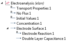
Model tree for the Electroanalysis interface in an EIS model.
Under Transport Properties, we can specify the diffusion coefficients of the redox species under consideration. We at least need the reduced and oxidized species for a single redox couple, such as the common redox couple ferro/ferricyanide, to use as an analytical reference. The Concentration boundary condition defines the fixed bulk concentrations of these species. The Electrode Reaction and Double Layer Capacitance subnodes for the Electrode Surface boundary feature contribute faradaic and nonfaradaic current, respectively. For the double-layer capacitance, we typically use an empirically measured equivalent capacitance and specify the electrode reaction according to a standard kinetic equation like the Butler-Volmer equation.
Note that we’re not referring to equivalent circuit properties at all here. In COMSOL Multiphysics, all of the inputs in the description of the electrochemical problem are physical or chemical quantities, while the output is a Nyquist plot. When analyzing the problem in reverse, we’re able to use an observed Nyquist plot from our experiments to make inferences about the real values of these physical and chemical inputs.
In the settings for the Electrode Surface feature, we represent the impedance experiment by applying a Harmonic Perturbation to the cell voltage.
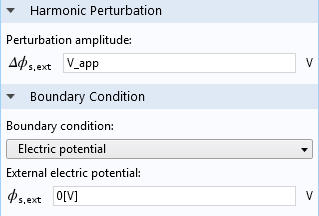
Settings for the Electrode Surface boundary feature in an EIS model.
Here, the quantity V_app is the applied voltage.
The harmonic perturbation is applied with respect to a resting steady voltage (or current) on the cell. In this case, we have set this to a reference value of zero volts. With more advanced models, we might consider using the results of another COMSOL Multiphysics model, one that’s significantly nonlinear for example, to find the resting conditions to which the perturbation is applied. If you’re interested in understanding the mathematics of the harmonic perturbation in greater detail, my colleague Walter discussed them in a previous blog post.
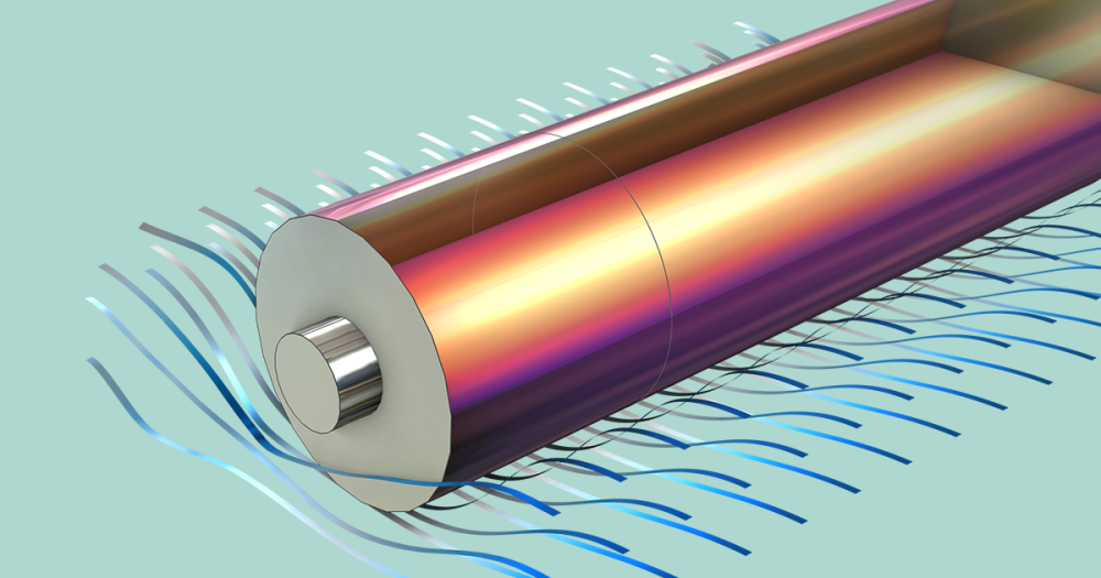
When studying lithium-ion batteries, for example, we can perform a time-dependent analysis of the cell’s discharge, studying its charge transport, diffusion and migration of the lithium electrolyte, and the electrode kinetics and diffusion of the intercalated lithium atoms. We can pause this simulation at various times to consider the impedance measured from a rapid perturbation. For further insight into the physics involved, you can read my colleague Tommy’s blog post on modeling electrochemical impedance in a lithium-ion battery.
Electrochemical Impedance Spectroscopy: The Simulation App
A frequent demand for electrochemical simulations is that they “fit” experimental data in order to determine unknown physical quantities or, more generally, to interpret the data at all. Even for experienced electroanalytical chemists, it can be difficult to intuitively “see” the physics and chemistry in the underlying graphs like the Nyquist plot. However, by simulating the plots under a range of conditions, the influence of different effects on the overall graph is revealed.
Simulation is helpful for analyzing EIS, but it can also be time consuming for the experts involved. As was the case with my old research group, these experts can spend more time writing programs and running models to fit data together with experimental researchers than on the science. Wouldn’t it be nice if all electrochemical researchers could load experimental data into a simple interface, simulate impedance spectra for a given physical model and inputs, and even perform automatic parameter fitting? The good news is that we can! With the Application Builder in COMSOL Multiphysics, we can create an easy-to-use EIS app based on an underlying model. As a model can contain any level of physical detail, the app provides direct access to the physical data and isn’t confined to simple equivalent circuits.
To highlight this, we have an EIS demo app based on the model available in the Application Library. The app user can set concentrations for electroactive species and tune the diffusion coefficients as well as the electrode kinetic rate constant and double-layer capacitance. After clicking the Compute button, the app generates results that can be visualized through Nyquist and Bode plots.
The EIS simulation app in action.
As well as enabling physical parameter estimation, this app is very helpful for teaching, since we can quickly change inputs and visualize the results that would occur in the experiment. A natural extension for the app is to import experimental data to the same Nyquist plot for direct comparison. We can also build up the underlying physical model to consider the influence of competing electrochemical reactions or follow-up homogeneous chemistry from the products of an electrochemical reaction.
Concluding Thoughts
Here, we’ve introduced electrochemical impedance spectroscopy and discussed some methods used to model it. We also saw how a simulation app built from a simple theoretical model can provide greater insight into the relationship between the theory of an electrochemical system and its behavior as observed in an experiment.
Further Reading
- Explore other topics related to electrochemical simulation on the COMSOL Blog


Comments (1)
Patricio Impinnisi
August 10, 2018Dear Ed, do the Comsol perform current perturbation EIS? (or just voltage EIS)