

This blog post is part of a series aimed at introducing the weak form with minimal prerequisites. In the first blog post, we learned about the basic concepts of the weak formulation. All equations were left in the analytical form. Today, we will implement and solve the equations numerically using the COMSOL Multiphysics simulation software. You are encouraged to follow the steps with a working copy of the COMSOL software.
Recapping the Basic Ideas
Recall that in the previous entry, we studied a simple example of 1D heat transfer at steady state with no heat source, where the temperature T is a function of the position x in the domain defined by the interval 1\le x\le 5.
The weak formulation turns the differential equation for the heat transfer physics into an integral equation, with a test function \tilde{T}(x) as a localized sampling function within the integrand to clamp down the solution. Integrating the weak form by parts provides the numerical benefit of reduced differentiation order. It also provides a natural way to specify boundary conditions in terms of the heat flux. For fixed boundary conditions, in terms of the temperature, the weak formulation uses the same mechanism of test functions and its natural boundary conditions to construct additional terms in the equation system.
In the end, we arrived at an exemplary equation that looks like this:
(1)
Here, the integrand on the left-hand side involves only the first derivative of the temperature, the first term on the right-hand side defines that the outgoing flux should be 2 at the left boundary (x=1), and the other two terms on the right-hand side together specify that the temperature should be 9 at the right boundary (x=5).
The Weak Form PDE Interface
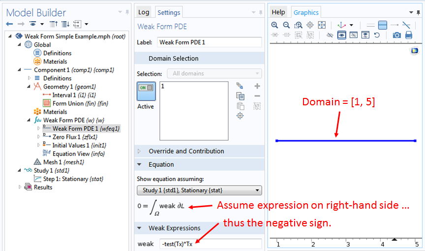
To implement Eq. (1) in COMSOL Multiphysics, we use the Model Wizard to create a new 1D model with a Weak Form PDE (w) interface (under Mathematics > PDE Interfaces) and a Stationary study. The dependent variable can be set to T to match the notation in our equation. For the geometry, we make an Interval between 1 and 5. The weak expression under the default “Weak Form PDE 1” node reads: -test(Tx)*Tx+1[m^-2]*test(T), where the first term corresponds to the integrand in our Eq. (1) and the second term corresponds to a heat source, which is not in our simple example and should be removed from the input field.
The weak expression now reads: -test(Tx)*Tx, where Tx is the COMSOL Multiphysics notation for \partial_x T(x), the first derivative of the temperature, and test(Tx) is the first derivative of the test function \partial_x \tilde{T}(x). The negative sign comes from the convention that the input field assumes that the expression is on the right-hand side of the equal sign (as seen in the “Equation” section of the settings window), while the integral in our equation is on the left-hand side.
The Weak Contribution Feature
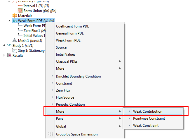
To implement the weak form terms on the right-hand side of Eq. (1) for the boundary conditions, right-click the Weak Form PDE (w) node. We see that there are built-in boundary features such as the Dirichlet Boundary Condition item, which is available in the pop-up menu for your convenience. However, since here we are interested in entering the equation ourselves, we hover the mouse over the item More in the pop-up menu and click on the item Weak Contribution in the next pop-up menu.
In the settings window for the “Weak Contribution 1” node under Boundary Selection, we select boundary 1 at the left end of the domain (at x=1). We then enter the weak expression as: -2*test(T) under the section Weak Contribution in the same settings window. This takes care of the first term on the right-hand side of Eq. (1), which specifies the outgoing flux to be 2 at the boundary x=1.
Fixed Boundary Condition
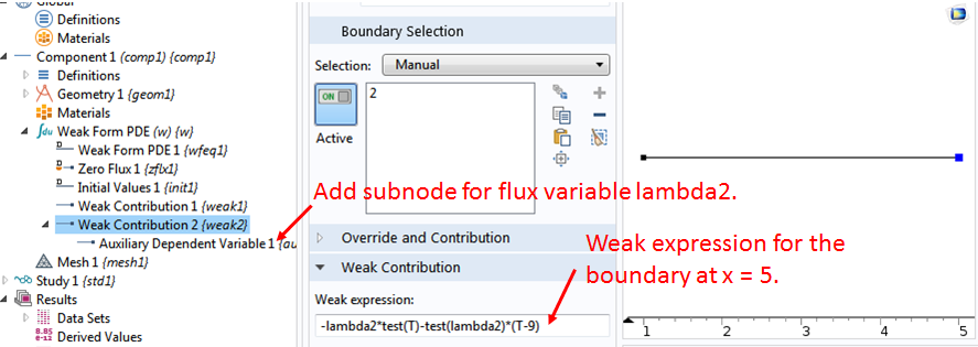
For the fixed boundary condition at x=5, where the last two terms on the right-hand side of Eq. (1) together specify that T=9, we create another “Weak Contribution” node at boundary 2 at the right end of the domain and an Auxiliary Dependent Variable subnode under it.
We enter lambda2 for the Field variable name in the subnode and then enter the weak expression as the two terms in Eq. (1): -lambda2*test(T)-test(lambda2)*(T-9)
Discretization
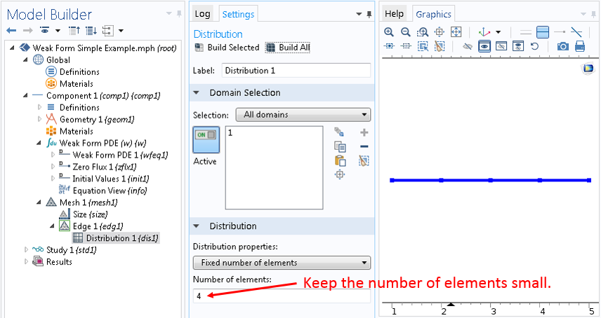
The COMSOL software discretizes the domain by creating a mesh. Let’s right-click the Mesh 1 node and select Edge and then right-click Edge 1 and select Distribution. Then, we set the “Number of elements” to 4 and click Build All. We intentionally keep the number of elements small to make it easier when we discuss the discretization in more detail later.
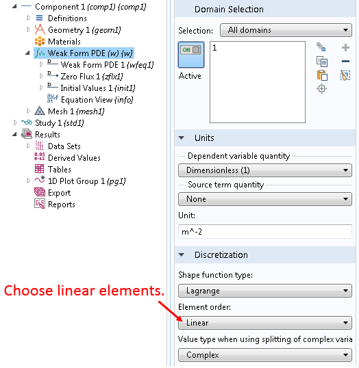
Also, under the Discretization section in the settings window for the Weak Form PDE (w) interface node, we set the “Element order” to Linear (click on the Show button under Model Builder and then the item Discretization in the pop-up menu to enable the Discretization section):
Compute the Solution in COMSOL Multiphysics
Now we are ready to click Compute and check whether the solution makes sense.
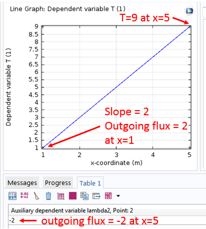
The solution gives a straight line within the domain, which is consistent with the temperature profile at steady state with no heat source. The slope of the line is 2, which is consistent with the boundary condition that the outgoing flux is 2 at x=1. The temperature is 9 at x=5, as specified by the fixed boundary condition. Since there is no heat source, the total heat flux going out of the domain should sum up to zero in the steady state. Thus, the outgoing flux should be -2 at x=5.
We readily verify this by making a point evaluation of the heat flux variable lambda2, as shown in the screenshot below:
Some readers may wonder whether it is always necessary to solve for the auxiliary variable lambda2, the so-called Lagrange multiplier, especially if it is not needed by the modeler and solving for it inevitably requires more computation. As we will see in the following posts, COMSOL Multiphysics provides alternative features and allows the user to decide whether or not to solve for the Lagrange multiplier.
Summary and Next Up
Today, we refreshed the concept of the weak formulation and implemented an exemplary weak form equation (1) in COMSOL Multiphysics. The resulting numerical solution behaves as expected from simple physical arguments.
In future blog posts, we will take a look “under the hood” to see how the weak form equations, such as Eq. (1), are discretized and solved numerically. We will see how the same problem can be solved in different ways and how different boundary conditions can be set up for different types of problems.
Stay tuned!

Comments (47)
Stefano Maffei
January 8, 2015Thanks a lot for this clear article. I am looking forward for the next ones.
Do you have a specific reference concerning finite elements/spectral elements that I can use to get more insights into these concepts?
Chien Liu
January 8, 2015Dear Stefano,
Thank you for your interest in this blog post. You may find the list of books below of interest.
Sincerely,
Chien
These books might be of interest for getting an in-depth knowledge of finite element analysis:
* T. J. R. Hughes, The Finite Element Method: Linear Static and Dynamic Finite Element Analysis, Dover Publications (2000)
* O. C. Zienkiewicz & R. L. Taylor, The Finite Element Method Set, Butterworth-Heinemann; 7th edition (2011)
* S.C. Brenner & L.R. Scott, The Mathematical Theory of Finite Element Methods, Springer; 3rd edition (2009)
For the application of the finite element method to partial differential equation in particular, these books might be of interest:
* K. Eriksson, D. Estep, P. Hansbo, C. Johnson, Computational Differential Equations, Cambridge University Press; 2nd edition (1996)
* C. Johnson, Numerical Solution of Partial Differential Equations by the Finite Element Method, Dover Publications (2009)
For fluid flow, this book has a section on comparisons between the finite volume method and the finite element method. It is also a good reference for different finite element types used for CFD:
* P. M. Gresho & R. L. Sani, Incompressible Flow and the Finite Element Method, Volume 2, Isothermal Laminar Flow, John Wiley & Sons (2000)
For Electromagnetics, especially high-frequency, this is an excellent reference:
* Jianming Jin, The Finite Element Method in Electromagnetics, Wiley-IEEE Press; 3rd edition (2014)
Camille Spingarn
February 3, 2015Ren Wenxi
February 7, 2015Dear Liu,
Thank you so much for your article about the weak form. I have been interested in the application of the weak form in structure analysis. Recently, i am trying to design a simple structure analysis module by weak form. But there is a problem in my code. I hope your help. The following is my code:
% Displacement field
% Dependent variables u, v
% Variables
E 1.44*10^4[MPa] % Young modulus
pr 0.2 % Poisson’s ratio
% Elasticity matrix
D11 E/(1-pr^2)
D22 E/(1-pr^2)
D33 E/(2*(1+pr))
D12 E*pr/(1-pr^2)
D21 D12
D23 0[Pa]
D32 0[Pa]
D13 0[Pa]
D31 0[Pa]
% Strain
ex ux
ey vy
exy 0.5*(uy+vx)
% Stress
sx D11*ex+D12*ey+2*D13*exy
sy D21*ex+D22*ey+2*D23*exy
sxy D31*ex+D32*ey+2*D33*exy
% Equations
-sx*test(ux)-sxy*test(uy) % X Direction
-sy*test(vy)-sxy*test(vx) % Y Direction
Ren Wenxi
February 7, 2015Look forward to your reply~
Chien Liu
February 9, 2015Hi Ren,
Thank you for contacting us on this. In this case we recommend that you please contact our support team for help. They can be reached at:
http://www.comsol.com/support
Best regards,
Chien
Stefano Maffei
February 18, 2015Hi Chien,
Let’s say I have a system of equations (in my case i have an eigenvalue problem). Then I multiply both equations by their corresponding test functions (say my variables are y and c), integrate by parts and apply the boundary conditions I have. Imagine after all I am left with something like:
\int [ weak form for y ] dx = [lambda*test(y)*yx]_x1
\int [ weak form for c ] dx = [test(c)*cx]_x1
where lambda is the eigenvalue (sorry if this looks complicated, I just think that with an example is better to talk about things). Imagine that somehow i have no informations about the derivatives in x0 (say i x1 everything vanishes).
My question is: these boundary terms have t be retained, as they might be important in adjusting the behaviour of the solution near x1. How should I treat them? Should I put in the weak contribution subnode
lambda*test(y)*yx + test(c)*cx
applied on x1?
Thanks
Chien Liu
February 18, 2015Hi Stefano,
Thank you for contacting us on this. In this case we recommend that you please contact our support team for help. They can be reached at:
http://www.comsol.com/support
Thanks!
Chien
Pu Zhang
April 16, 2015Very nice blog post! So is this possibility of inspecting system matrix a new feature in COMSOL 5?
Chien Liu
April 17, 2015Hello Pu,
Thank you for the comment. You were probably referring to this entry:
http://www.comsol.com/blogs/implementing-the-weak-form-with-a-comsol-app/
The possibility of inspecting the system matrix is not new. In fact it has been available to users from the beginning.
Of course the Application Builder is a brand new feature in COMSOL 5.0 (and further enhanced in 5.1). We believe the users’ productivity can be greatly improved by COMSOL Apps, as illustrated in the above blog post (and many others).
Chien
Chien Liu
April 17, 2015In the previous message I forgot to add the link to other blog posts on COMSOL Apps. They can be found here:
http://www.comsol.com/blogs/category/all/applications/
jackshine ma
June 18, 2015Dear Chien Liu,
Very glad to learn from your blog on Weak form of comsol and it’s a very good blog specifying on weak form that merely introduced detailedly anywhere. However, I wonder that why there is a 2-order differential in integrand but only 1 time integral on the left of equation 1. If like this, the calculating result of left term would be in a differential form, which is not like the right polymial.
Chien Liu
June 22, 2015Hi jackshine ,
Thank you for the comments.
I’m not sure I understand your question since there is no time integral in equation 1.
The integrand should be interpreted as having parenthesis as follows: (dx T) (dx T_test).
Hope this help clarify the equation.
Chien
Vishwas Nesarikar
October 22, 2015Can you please provide derivation of Eqn (1) ? Thx
Chien Liu
October 22, 2015Dear Vishwas,
The derivation is in this previous blog post:
http://www.comsol.com/blogs/brief-introduction-weak-form/
Hope this helps.
Sincerely,
Chien
Parth Swaroop
April 11, 2016Dear Chien,
Implementation of this weak formulation and use T_lm is also presented in example of “Tin Melting Front” module provided by comsol. In this example the movement of the melting phase is implemented as :
T_lm[W/m^2]/(rho*DelH)
i guess [W/m^2] is used make the units m/s ( normal velocity of the prescribed mesh ).
how do i know that this expression actually evaluates the difference in flux at the interface and not the temperature profile.
from physics, the expression for normal velocity is
ΔH_fus ρ v_n= ϕ_l- ϕ_s
Parth
Chien Liu
April 12, 2016Dear Parth,
In the Tin Melting Front example, the variable T_lm is the heat flux and it plays exactly the same role as the variable lambda2 in the blog post.
The formula for the normal mesh velocity v can be understood in the following way:
v * rho = rate of melting
DelH = latent heat of fusion
therefore
v * rho * DelH = heat flux = T_lm
Does this make sense?
Sincerely,
Chien
Jorge Yannie
April 17, 2016Hello Chien,
Great post once again! Looking forward to all your Equation-based post! It is my main goal to learn in Comsol!
Like it lot!
Puneeth Banisetti
April 23, 2016Hello Chein,
Thanks a lot for a very informative blog post. I thoroughly enjoyed it. I want to know how we can implement this technique when we have some normal boundary conditions for 3D problems such a parallel plate rheometer. How do we incorporate the boundary condition (T.n).n=0 and what exactly do we take n when we are using cartesian coordinates since n here will be in the radial direction.
Could you also please post the link for the continuation of this blog post.
Regards,
Puneeth
Chien Liu
April 26, 2016Dear Puneeth,
You can find related posts by typing in “weak form” in the “Search Blog” search box above.
For normal variables please refer to the COMSOL Reference Manual > Global and local Definitions > Predefined and Built-in Variables > Geometric Variables and Mesh Variables > Tangent and Normal Variables.
Sincerely,
Chien
Edward Smith
June 23, 2016Hi
I’ve been trying to implement this example but cannot select the points at either end of the interval. It only lets me select the whole domain. I suspect I have done something wrong in Geometry.
Thanks
Chien Liu
June 23, 2016Dear Edward, when creating a weak contribution on a boundary, make sure to select the item from the group of boundary features, not the domain features. It sounds like you selected the latter. You may find the 2nd screenshot in the blog post helpful.
Sincerely,
Chien
Edward Smith
June 23, 2016Hi
Thanks for the reply.
What a fool I am 🙂
Ted
Edward Smith
June 23, 2016I am trying to use the Laminar flow subset of the N-S equations, and want to prevent any pressures going negative. Can I do this with a weak contribution?
Iris Zhou
November 14, 2016Hi Chien,
Thanks for your blog, and it is really nourishing!
Right now I am working with Frequency domain Wave-optics Module (ewfd2). I am using electric field as the input boundary condition, and with numerically calculated data from an eigenfrequency solver (ewfd.E). I want to put both electric fields and their derivatives into the boundary condition, and I thought this blog is quite relevant.
Should I use electric field with Weak Constraints? If so, how should I put numerical derivative, e.g., d(ewfd.Ex,x), to the Weak Constraints?
Looking forward for your reply! Thanks in advance!
Iris
Bridget Cunningham
November 15, 2016Hello Iris,
Thank you for your comment.
For questions related to your modeling, please contact our support team.
Online support center: https://www.comsol.com/support
Email: support@comsol.com
Best,
Bridget
akshay phadnis
January 26, 2017Dear Chien,
Thanks for this article. It’s a great help. There is no other documentation about weak form implementation in COMSOL. I am trying to model the polymer swelling using solid mechanics equation – div(S)+b=0. When I convert this into a weak form, I get the expression in terms of deformation matrix. Now comsol weak form interface cannot take deformation tensor as input, it has to be specified in terms of displacement. Do you have any suggestions on how I can proceed with implementing solid mechanics problem using weak form ?
Bridget Cunningham
January 26, 2017Hello Akshay,
Thank you for your comment.
For questions related to your modeling, please contact our support team.
Online support center: https://www.comsol.com/support
Email: support@comsol.com
Best,
Bridget
Manal Badgaish
February 19, 2017Dear All,
I have the following 1D PDE system:
u_tt= c^2 *u_xx,
u(x,0)=u_t(x,0)=0, (initials conditions)
m* u_tt(0,t)= a*PB(t)+rho*c^2*a*u_x(0,t)-D1*u(0,t)- D2*u^2(0,t)-D3, (boundary condition1)
u_t(Let)=-c*u_x(L,t). (boundary condition2)
I want to find the solution at x=0 only, i.e I need to solve for u(0,t).
Is it possible to implement this pdf system in comsol with this nonlinear complicated boundary condition at (x=0)? Can any one tell me the steps of doing it, and how I write the weak form of this complicated boundary conditions.
Thanks,
Manal
Bridget Cunningham
February 21, 2017Hello Manal,
Thank you for your comment.
For questions related to your modeling, please contact our support team.
Online support center: https://www.comsol.com/support
Email: support@comsol.com
Best,
Bridget
Konark B
May 16, 2017Hi,
What is the significance of negative sign in implementing weak form? Should it work equally if we don’t write negative sign since LHS is zero?
Chien Liu
May 16, 2017Dear Konark,
As long as the sign convention in your design is consistent (remember that there can be more than one weak contribution in general), you are free to choose the most convenient one for you.
Sincerely,
Chien
eric malitz
August 4, 2017If we have multiple weak equations, i.e. a mixed finite element method, how would we code a boundary integral in each equation individually? The “weak contribution” options don’t seem to allow this specification.
Chien Liu
August 7, 2017Dear Eric,
The Weak Contribution feature’s input field allows any combination of multiple field variables, or if you prefer you can use multiple Weak Contribution nodes in the Model Builder tree structure. For any specific question please feel free to contact us at support@comsol.com or http://www.comsol.com/support
Sincerely
Chien
Ngo Dinh Nhan
August 17, 2017Dear Dr.Chien Liu
I followed your steps in the instructor, but actually, the 1D plot was not same as your plot.
I have attached my plot in this link ( google photo )
https://goo.gl/photos/ueqVhn7CY9USQumR6
Best regards
Chien Liu
August 22, 2017Dear Ngo,
It looks like you may have forgotten to set the B.C. at x=1.
Sincerely,
Chien
Vaidehi Oruganti
February 1, 2018Dear Dr.Chien Liu,
I am trying to implement weak form modelling to solve a benchmark problem of flow between two flat plates (parabolic profile).
I have trouble computing the velocity and pressure fields. I am ending up with the error that system matrix is zero and an under-specified problem.
Method to solve flow between plates:
(1) Two weak form PDE interfaces. One PDE solves for velocity field (momentum equation) and the other solves pressure field (continuity equation)
Weak form PDE (1)
x-comp: mu*(test(ux)*ux+test(uy)*uy)+px*test(u)
y-comp: mu*(test(vx)*vx+test(vy)*vy)+py*test(v)
BC(1) : No Slip -u*test(-u)-v*test(-v)
Constraints are: [-u, -v]
Constraint Force: [-test(u),-test(v)]
For inlet and outlet: n.T_stress= -(p_ext)n
p_ext at inlet is set to 2 [Pa] gauge and p_ext at outlet is zero
Weak form of continuity:
test(p)*(ux+vy)
2 dirichlet conditions , p=2 [Pa] at inlet and p=0[Pa] at outlet are imposed.
The simulation does not work. Can you throw some light on what I am doing wrong?
Caty Fairclough
February 1, 2018Hi Vaidehi,
Thanks for your comment.
For your question, please contact our Support team.
Online Support Center: https://www.comsol.com/support
Email: support@comsol.com
Vaidehi Oruganti
February 1, 2018Dr. Chien Liu,
I tried contacting the COMSOL support about the issues I have, but I heard that they cannot provide assistance on weak form modelling to people having academic licenses (which I have) Therefore, I request you to throw some light on the problem. I did read the weak form documentation and all of your blog posts on weak form modelling.
Thank you Sir.
Vaidehi Oruganti
February 1, 2018I tried contacting COMSOL support but they say they cannot offer support on weak form modeling. This is the reason I am trying to reach out to you.
Thank you Sir.
Vaidehi Oruganti
February 1, 2018Dear Caty Fairclough,
The following is the reply I received from COMSOL support just now, about the above question.
“Dear Vaidehi,
Thank you for contacting COMSOL Support.
The question being asked here pertains to equation based modeling.
Additionally, the application of this equation based modeling is recreating
an existing fluid flow interface. These types of questions do fall outside
the scope of the technical support we provide.
Best Regards,
COMSOL Technical Support”
So, you see COMSOL support does not answer any questions about equation based modelling. Therefore, I am trying to get some assistance here.
shi tan
April 15, 2019Dear Dr.Liu
I am using version 5.4, what are detailed steps to get the value of lambda2?
Chien Liu
April 16, 2019Dear Shi, The steps should be the same. Please contact support if you need further assistance. Sincerely, Chien
Avishai Benyamini
January 4, 2021Dear Chien Liu,
Thanks for writing and maintaining the blog.
I have a question regarding equation (1).
If instead of a constrain for T_2=9 I had a constrain \partial_n ( T_2 ) = 9 (with n the normal vector on the surface and \partial_n denotes a partial derivative at that direction), should the lambda_2 term have a similar partial derivative? That is in equation (1) we will have instead:
-lambda_2 * \partial_n ( \tilde{T}_2 ) – \tilde{\lambda}_2 * (\partial_n ( T_2 ) – 9)
If not, what is the right way to formalize this?
Thanks!
Chien Liu
January 5, 2021 COMSOL EmployeeDear Avishai Benyamini, Thank you for the question. What you wrote looks like a Neumann boundary condition similar to the one on boundary 1 in the example. If there are any further questions please feel free to contact us at COMSOL support. Sincerely, Chien
Space lab
July 27, 2023Hi, Dr. Liu:
If the PDE is of third order, should we reduce it until we end up with terms involving first order derivative terms. or is it enough to get an equation involving second order terms after applying integration by parts.
Nicolas Ruyssen
January 31, 2024Dear Chien Liu,
thank you for this very clear article, and in particular the explanations about the boundary integral implementation.
I would like to know (if possible), how could I implement a periodic boundary condition using only a weak contribution ?
Thank you by advance