

RF coil technology is ubiquitous throughout the world and serves as a major component of technologies, from medical equipment to wireless connectivity. It is important to ensure that the coils contained within these devices transmit information from a source to its destination properly.
What Are RF Coils?
RF coils are electromagnetic (EM) coils that transmit and receive radio frequency (RF) signals. The transmitter coil generates EM fields, while the receiver coil, as the name suggests, receives them. RF coils can be found in various devices, such as magnetic resonance imaging (MRI) systems, for example. In MRI scanning equipment, radio waves and uniform, strong magnetic fields are used to form images of the patient’s anatomy. RF coils are also used for impedance matching of predominantly capacitive devices such as RF plasma reactors for semiconductor manufacturing.
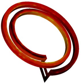
An RF coil.
An important characteristic of an RF coil is its frequency response, especially the resonance frequency; the frequency at which the reactive part of the impedance between the input and output of a coil becomes zero.
Finding the Resonance Frequency of an RF Coil
One of our introduction tutorials for RF modeling involves an RF coil model. Using COMSOL Multiphysics and the RF Module, we can analyze the signal strength of an RF coil by solving for its resonance frequency and Q factor, among other properties.
Let’s have a look at a copper coil made of two turns.
Version 1
First, we want to find the fundamental resonant frequency, i.e. the lowest frequency of the coil. We do so by performing an eigenfrequency analysis of the model geometry that is shown below.
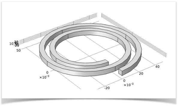
RF coil geometry.
We will consider the coil to be a perfect electric conductor, so we will only need to solve the eigenfrequency equation for the electromagnetic waves in the surrounding air domain.
Version 2
Next, we want to find the lowest eigenfrequency of the model. We use a lumped port to apply a time-harmonic driving port voltage between the two ends of the coil. The port is assigned a 50 Ω external cable impedance and a driving voltage of 1 volt (V).
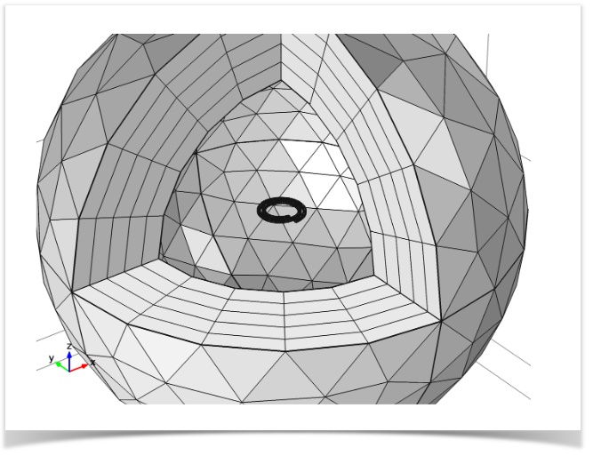
Mesh used in a driven version of the model. A slice is cut out and the air domain is made invisible to show the coil.
Based on our results in Version 1, we run our model through a range of frequencies around the resonance frequency. After conducting our eigenfrequency analysis, we find that the lowest eigenfrequency is 180 MHz.
Then, we can obtain the distribution of electric and magnetic fields at this resonance:
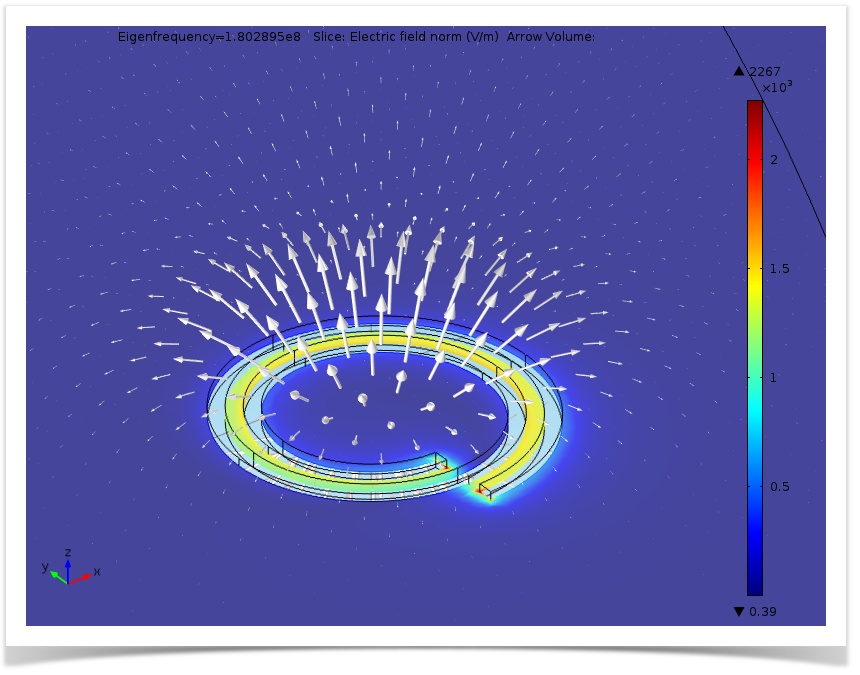
Simulation of the electric field (slice) and magnetic flux density (arrows) at the fundamental resonant frequency.
Because this particular coil transmits or receives signals through resonance, it’s important to determine the Q factor, i.e. the quality factor. The Q factor is a dimensionless parameter that describes how under-damped an oscillator or resonator is. It is determined by the ratio of peak frequency to the full width at half maximum for the frequency response of the coil impedance. A higher Q factor indicates that oscillations die out more slowly and the coil will be more efficient at the resonance frequency. However, it also indicates that the coil has a narrow bandwidth, so it will be more sensitive to any frequency mismatch.
The Q factor can be extracted by plotting the input impedance versus frequency. Electrical impedance describes the total resistance to an alternating current by an electric circuit. Using our previous results, we continue our analysis and solve for the impedance of the model across a range of frequencies around the resonant frequency of 180 MHz.
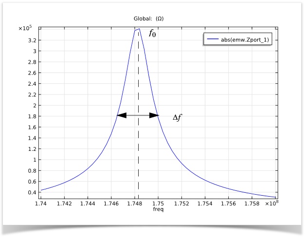
Plot of input impedance magnitude versus frequency, where f0 is the peak or resonance frequency and Δf is the full width at half maximum.
The Q factor for our model is around 300, which confirms that the system is not under-damped and will exhibit sufficient frequency bandwidth.
Model Download
- The tutorial model shown here can be accessed from both the Model Gallery and the Model Library with step-by-step instructions and an MPH-file.


Comments (5)
Dayang Rogayah
April 24, 2017Hye,
i try the RF coil tutorial, i want to know why the S parameter at positive value and goes higher value. As i know the s parameter value indicates the return loss and it should be low dB value(the negative value is better).Thank You
Caty Fairclough
May 3, 2017Hi Dayang,
Thanks for your comment!
For your question, please contact our Support team.
Online Support Center: https://www.comsol.com/support
Email: support@comsol.com
Dayang Rogayah
May 4, 2017Hye, Caty..
Okay, Thank you.
khalesh shaik
May 27, 2017Computing of eigenfrequency is very slow and showing error “out of memory during assembly”. any way to solve it.
Caty Fairclough
June 6, 2017Hi Khalesh,
Thank you for your comment.
For your question, I’d suggest contacting our Support team.
Online Support Center: https://www.comsol.com/support
Email: support@comsol.com