
The COMSOL Multiphysics® software is often used for modeling the transient heating of solids. Transient heat transfer models are easy to set up and solve, but they aren’t without their difficulties to work with. For example, the interpretation of their results can confuse even the advanced COMSOL® user. In this blog post, we’ll explore a model of a simple transient heating problem and use it to gain an in-depth understanding of these nuances.
A Simple Transient Heating Problem
Figure 1 shows the modeling scenario that is the topic of discussion for this blog post. In this scenario, a spatially uniform heat load is applied to a circular region on the top surface of a cylinder of material that has a uniform initial temperature. The magnitude of the load is initially high, but steps down after some time. In addition to this applied heat load, a boundary condition is included to model thermal radiation from the entire top surface, which cools the part back down. It’s assumed that the material properties (thermal conductivity, density, and specific heat) and the surface emissivity remain constant over the expected temperature range. It’s also assumed that no other physics come into play. The objective of this model is to be able to use it to compute the temperature distribution within the material over time.
A similar modeling scenario is featured in our Laser Heating of a Silicon Wafer tutorial model, but let’s keep in mind that the lessons discussed here are applicable to any case involving transient heating.
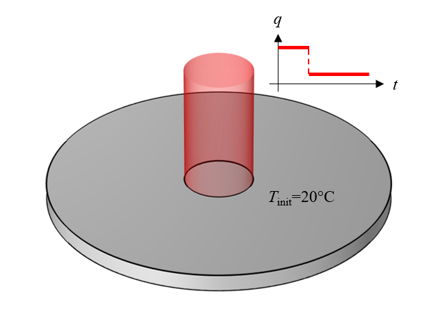
Figure 1. A cylinder of material with a heat source over the top surface.
Although it’s tempting to begin setting up our model by drawing the exact geometry shown in Figure 1, we’ll start with a simpler model. In Figure 1, we can see that the geometry and load is axially symmetric about the centerline, so we can reasonably infer that the solution will also be axially symmetric. Therefore, we can simplify our model to the 2D axisymmetric modeling plane. (Get an introduction to using symmetry to reduce model size here.)
The heat flux is uniform over a circular region in the middle. The simplest way to model this is to modify the geometry by introducing a point on the boundary of our 2D domain. This point partitions the boundary into heated and unheated sections. Adding this point to the geometry ensures that the resultant mesh is exactly aligned with this change in the heat flux. Keeping all of this in mind, we can create a computational model (Figure 2) that is both 2D axisymmetric and equivalent to the 3D model.
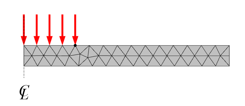
Figure 2. The 2D axisymmetric model that is equivalent to the 3D model. Shown with the default mesh.
The case we’re considering also includes an instantaneous change in the magnitude of the applied heat flux; at t = 0.25 s it goes to a lower value. Such step changes to the loads should be addressed by using the Events interface, as described in this Knowledge Base entry on solving models with step changes to loads in time. In short, the Events interface tells the solver exactly when the change in the load occurs and the solver will adjust the time step accordingly. We might also like to know what time steps the solver is taking so that we can modify the solver settings to output the results at the steps taken by the solver, and we can then plot the temperature of the point in the top center of the part, as shown in Figure 3.
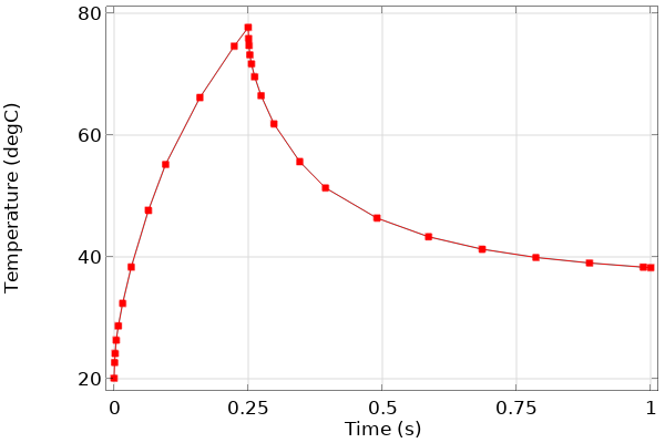
Figure 3. Plot of the temperature over time at one location, with points showing that the steps taken by the solver are shorter near the abrupt changes to the loads.
Next, we rerun the model with different values for the solver relative tolerance and compare it in a plot (Figure 4). This type of plot shows us that the solutions converge rapidly toward the same values as the tolerance is made tighter, as expected.
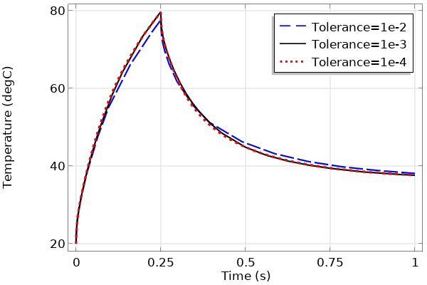
Figure 4. Plot of the temperature at one point over time, solved with different relative tolerances.
Another quantity that can be evaluated here is the total amount of energy entering the domain. We can integrate the expression for the total heat flux, ht.nteflux, over the boundaries, and we can use the timeint() operator to integrate over time to get the total energy. The results of this integral are tabulated below for increasing time-stepping relative tolerance. (Tip: Learn more about computing space and time integrals in this Knowledge Base entry, and learn more about computing energy balances in this blog post on how to calculate mass conservation and energy balance.)
| Solver Relative Tolerance | Time-Integral of Flux into Modeling Domain (J) |
|---|---|
| 1e-2 | 32.495 |
| 1e-3 | 32.469 |
| 1e-4 | 32.463 |
What we observe from the data is that the total energy into the system is actually almost independent of time-stepping tolerance. At first glance, this seems to be a fantastic validation of our model. However, it’s important to point out that what we’re observing here is the fundamental mathematical property of the finite element method (FEM). In short, the total energy will always balance very well. This does not mean that there are no errors in the model, the errors just appear in different places…so let’s go looking for them now.
Errors: They’re Easy to Make, but Hard to Define
We should pause here and address with great care one word in the above paragraph, the word error, which is often used in the world of modeling and simulation without context or sufficient precision. In the rest of this section, we’ll present a few detailed descriptions of different errors that can appear in a variety of modeling cases. (If you want to skip ahead to the section related to errors in our model, click here.)
Input Errors
An input error, as its name suggests, is an error in the input of a model, such as when the material properties are not entered correctly or when the geometry is drawn wrong. One of the most pernicious input errors is an error of omission, such as when a boundary condition is forgotten. Input errors are distinct from uncertainties in the input, which, for example, can occur when the exact material properties aren’t known. The former can only be addressed by careful bookkeeping, while the latter can be addressed via the Uncertainty Quantification Module. For our example, we’ll say that there are no input errors or uncertainties.
Geometry Discretization Errors
A geometry discretization error arises when discretizing the geometry via the finite element mesh, especially when meshing nonplanar boundaries. These errors decrease with increasing mesh refinement and can be evaluated without actually solving a finite element model. Since our 2D axisymmetric modeling domain has no curved boundaries, we’ll not have to worry about this type of error either.
Solution Discretization Errors
A solution discretization error is a result of the fact that the finite element basis functions cannot perfectly represent the true solution field and its derivatives within this domain. It’s fundamentally present within the finite element method. This error, which is intrinsically linked to the geometric discretization error, is always present, and is always reduced with mesh refinement for any well-posed finite element problem.
Time-Stepping Errors
Understanding error propagation in a time-domain model is fairly involved. For the purposes of this blog post, it’s sufficient to say that any errors that are introduced or that are already present at any one time step will propagate forward, but for the type of diffusive problem we’re addressing here, they will decay. This type of error is always present, and the magnitude of these errors is controlled by both the time-dependent solver tolerance and the mesh.
Interpretation Error
There’s another type of error that is a bit more qualitative: the interpretation error. These errors occur when the meaning of the results and how they were produced are not precisely understood. One of the most famous of these is the singularity at sharp corners, a situation which often arises in structural mechanics as well as in electromagnetic field modeling. Interpretation errors arise especially often when there are input errors present. So if you are ever unsure of your results, it’s important to go back and double-check (or even triple-check!) all inputs to your model.
This list is not complete. For example, we could also talk about the numerical errors due to finite precision arithmetic of the linear system solver, the nonlinear system solver, and the numerical integration error. However, these, and other types of errors, are essentially always much smaller in magnitude.
With that set of definitions out of the way, we are now ready to return to our model.
Tracking Down Errors in Space and Time
So far, we have looked at the solution at one point in the model and observed that the solution appears to converge very well as we refined the time-dependent solver relative tolerance, so already we should have understood the idea that tightening the time-dependent solver relative tolerance will decrease time-stepping error. Now let’s look at the spatial temperature distribution. We’ll start with the temperature along the centerline, and for the loosest tolerance of 1e-2 look at the solution for the initial time as well as the first time step taken by the solver, in the plot below.
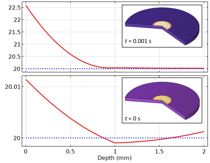
Figure 5. Plot of the centerline temperature for the initial time and the first time step.
From the initial value plot, we can see that the temperature along the centerline does not agree with the specified initial temperature — in some places it’s even lower than the initial value. This is due to the fact that COMSOL Multiphysics uses so-called consistent initialization, which adjusts the solution field at the initial time to be consistent with the boundary conditions and initial values at the initial time. Consistent initialization involves taking an additional very small artificial time step that we can think of as occurring over zero time. Consistent initialization can be turned off within the solver settings for the initial time step, as well as within the Explicit Events and Implicit Events features, but this should be done with some caution. In a more general multiphysics model, especially ones involving fluid flow, it can be more robust to leave it enabled by default, so we’ll address that case here.
The way to think about consistent initialization in this context is that it adjusts the temperature field to be in agreement with the applied loads and boundary conditions. Since the applied heat load is initially nonzero, the gradient of the temperature field, which is proportional to the heat flux, must be initially nonzero as well. We also need to consider that this field is discretized using the finite element basis functions. Along the centerline, these basis functions are polynomials, but a polynomial cannot exactly match the true solution; therefore, what we end up with after the consistent initialization step is a solution that will slightly over- and under-shoot the expected result. From the first time step solution, we can also see that the temperature on the far side of the part is already going up, which is unexpected. Although these variations from our expectations are very small in magnitude, we would like to minimize them.
Before modifying our model to reduce these solution discretization errors, let’s apply a little bit of physical intuition to the problem. At the start of the simulation time, the temperature distribution along the centerline will be quite similar to the solution for a modeling scenario that involves the simulation of heat transfer through a one-dimensional slab. An analytic solution already exists for this type of modeling scenario, which is often covered in many books on heat transfer analysis. (In fact, this example is used as the cover illustration of one of the textbooks on my desk, the Fundamentals of Heat and Mass Transfer.)
For brevity, we’ll skip going through the analytic solution and will instead just state the result: When you apply heat to the surface part, the temperature at the surface will start to rise, and eventually the interior region will get warmer as well. Note that it takes more time for points farther away from the boundary to heat up. The temperature within the slab is not going to vary homogeneously: At points further within the interior, it will take a longer time before the temperature starts to change as compared to points nearer to the surface. It’s important to note that the spatial temperature variations will smooth out over time due to the diffusive nature of the heat transfer equation. With this understanding, lets return to our model and see how to improve it.
In short, in order to minimize this solution discretization error, we need to mesh more finely where the fields will vary significantly. Based on our intuition (or the analytic solution, if we want to look it up), we know that the fields vary significantly very close to the surface and in the direction normal to the boundary but get more smoothed out within the interior. This is exactly the kind of situation that calls for boundary layer meshing, which creates thin elements normal to boundaries, as shown in Figure 6.
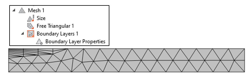
Figure 6. The meshing sequence is modified by adding a boundary layer along one boundary on the top of the wafer.
We now can rerun the simulation and plot the solution at the initial time and next time step.
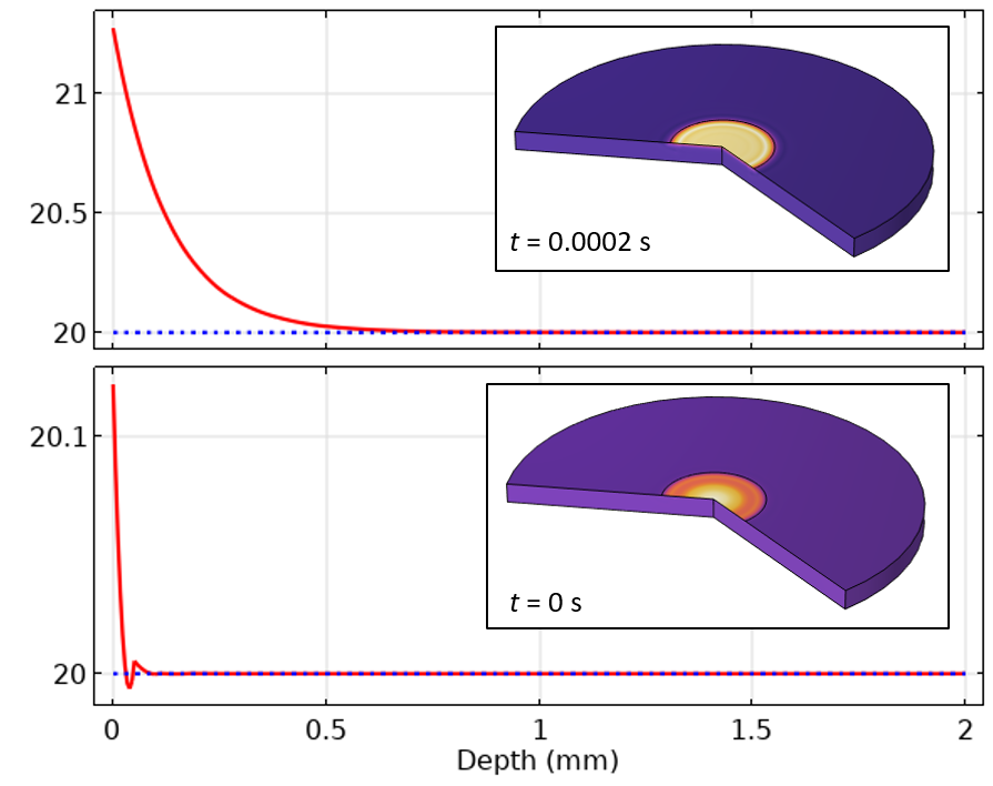
Figure 7. Plot of the centerline temperature at the initial and first time steps when using the boundary layer mesh.
In Figure 7, we can observe that the undershoot in temperature at the initial value is much more localized in space. It turns out that using a more refined mesh also results in the time-dependent solver taking smaller time steps. So, with this refinement of the mesh, we’ve reduced both spatial discretization and time-stepping errors.
We can also look at the results along the top boundary of the modeling domain, representing the temperature distribution over the exposed surface. In Figure 8, this is shown plotted for the initial time and first time step using a tolerance of 1e-2. In these plots, we can observe a quite dramatic oscillatory field in space. This is a symptom of spatial discretization. Keep in mind that our heat load experiences a step change in magnitude along the radial axis, and what we’re observing here is somewhat akin to the Gibbs phenomena.
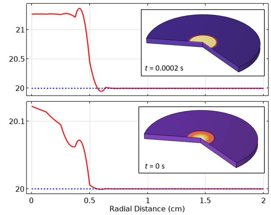
Figure 8. Plot of the temperature along the top surface at the initial value and first time step, using boundary layer mesh.
The solution is similar to before, but now we have to refine the mesh in the locality of the transition. For this problem, it’s possible to apply a finer Size setting to the delineating point, resulting in the mesh shown below.

Figure 9. Plot of the Mesh settings and mesh, with a smaller mesh size applied at the point delineating the heat load distribution.
From the temperature results in Figure 10, we see that the oscillations in the solution are now reduced and do not propagate as much in space or time. Even with a solver relative tolerance of 1e-2, the solution is already much improved.
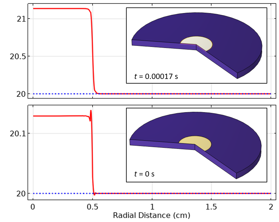
Figure 10. After refining the mesh, and using a relative tolerance of 0.01, the temperature along the top surface at the initial value and first time step is much more accurate.
It’s possible to continue this exercise using even more mesh and solver tolerance refinements. But through the refinements that we’ve done so far, we can already start to see that the errors diminish rapidly — and even the errors that are still present get smoothed out in both space and time due to the diffusive nature of the transient heat transfer equation. In fact, we should likely spend just as much effort investigating the effects of uncertainties in our model inputs.
What Else Can Come into Play?
In this example, the heat load applied across the boundary does not move in time, so the approach of partitioning boundaries is reasonable. If the heat load distribution were to move, then the mesh entirety of the heated surface would need to be more refined. (Explore three approaches to modeling moving loads and constraints in COMSOL® here.)
Earlier in this blog post, it’s mentioned that the material properties are assumed to be constant with temperature and do not depend on any other physics. This is a significant simplification, as all materials properties change with temperature. Materials could even experience phase change, such as melting. Phase change can be modeled several different ways, including with the Apparent Heat Capacity method, which uses a highly nonlinear specific heat to account for the latent heat of phase change. We could also easily envision this being a multiphysics problem, such as one involving an equation for thermal curing, or even a material nonlinear electromagnetic heating problem. In such cases, we would need to monitor the convergence of not just the temperature field, but all other field variables being solved for, and possibly even their temporal and spatial derivatives. These cases may all require a very fine mesh everywhere in the modeling domain, so the lessons from this simple situation do not carry over. However, even when meshing and solving much more complicated models, it’s always good to keep the simplest possible case in mind (even if it only serves as a conceptual starting point).
In addition, we should emphasize that this article is only about the time-varying heating of a solid material. If there is a moving fluid, the governing equations will change substantially; the meshing of fluid flow models is a separate and relatively more complex topic. For wave-type problems, the selection of mesh and solver settings becomes a fair bit simpler.
Closing Remarks
In this blog post, we have gone over a typical heat transfer modeling problem. We have observed that there are certain errors that appear in the solution near abrupt changes to the loads, in both space and time. Readers should now have an understanding as to what kinds of errors these are and know that they are an inherent consequence of the finite element method which is, like all numerical methods, only an approximation of reality. Although these errors can appear significant, their magnitude decays in space and time due to the diffusive nature of the transient heat transfer equation. We have shown that mesh refinement will reduce spatial discretization errors, which implicitly has the effect of reducing time-stepping errors. Lastly, we discussed how time-stepping errors can be further reduced with solver relative tolerance refinement.
It’s also worth giving an even briefer summary: If you are primarily interested in the solution after a relatively long time, it’s perfectly acceptable to use a quite coarse mesh and default solver relative tolerance. On the other hand, if you are interested in the short-duration and small-scale temperature variations, you must study both solver relative tolerance and mesh refinement.
With this understanding, we can avoid making interpretation errors. This will enable us to build more complex models from simple models with confidence and ease.
Next Step
Try the model featured throughout this blog post yourself by clicking the button below, which will take you to the Application Gallery:

Comments (18)
Ivar KJELBERG
December 17, 2022As usual, a great Blog, I like the discussion about “Errors” 🙂
What I still do not understand (probably neither do you) why COMSOL Multiphysics(r) is not the reference tool for all teaching and by most industries ? Because, if you understand Physics, and know COMSOL, you have all means to check your results, to avoid errors, something lacking in such details in most of the “old” modelling tools I have used over the last decades …
Just a pity my time is soon over and out, so fun to play with Physics with COMSOL …
Thanks for the great updates in the new release 🙂
Sincerely,
Ivar
Walter Frei
December 19, 2022 COMSOL EmployeeHi Ivar,
Thank you, my friend. 🙂
There is indeed a great deal I do not understand. And getting analysts to think about their numerical models in a careful way can be a near-Sisyphean task, and yet somehow I still enjoy it after all these years 😉
All the Best,
Walter
Helger van Halewijn
December 19, 2022I agree with Ivar, the content of this Blog is very interesting and enlightning. I will use this as a bases to explain systematically what is important to take into account in a “simple” thermal simulation.
Regards,
Helger van Halewijn.
Walter Frei
December 19, 2022 COMSOL EmployeeThank you Helger!
Jay Puckett
December 21, 2022Walter, very nice discussion. It is good to see an article on the basics using a simple model. Great reading for any introductory finite element class. Jay
Walter Frei
January 4, 2023 COMSOL EmployeeThank you Jay!
Mohamed Issa
December 21, 2022Impressive blog! I wonder if you provide dedicated courses where I can register for myself as a PhD student to use COMSOL in my thesis simulation. If so please guide me to where I can join such courses? Thank you.
Walter Frei
January 4, 2023 COMSOL EmployeeHello Mohamed,
COMSOL’s offers courses here:
https://www.comsol.com/events/training-courses
You’ll also find a lot of self-guided content within our Learning Center, Blogs, and Knowledgebase articles.
Happy Modeling!
Fabio Pulvirenti
December 21, 2022Hi Walter
Great blog! To answer Ivar’s question…. COMSOL has for sure the possibility to become the reference tool for many industries but I think that, besides new features, more blogs like this should be created basing on the opinion of the majority of the customers to identify which topics are wanted the most. I have been using COMSOL for 17 years now and I have been part of COMSOL family too, and I have seen situations where a feature was already part of COMSOL package but the application of that feature was not sufficiently known. In geophysics for example, the subnode feature “predeformation”, solved most of the issues that many research institutes were struggling with. Many switched to COMSOL(NASA, Stanford University, San Diego, and others). I would suggest COMSOL to better monitor what people want to solve.Maybe with periodic surveys? Sometime the features are already there but are unknown to most of the people and blog articles like this are helpful and very wanted! There is a huge interest for example from the tyre industry but no blogs yet. Hope to see something in the near future. Wish you the best of success with incoming challenges!
Sincerely,
Fabio.
Walter Frei
January 4, 2023 COMSOL EmployeeThank you Fabio!
Yaohui Chen
January 4, 2023It is enlightening. Even in industry’s engineer community, it is rare to have such awareness on the sanity check details on a “simple” thermal modeling.
Walter Frei
January 4, 2023 COMSOL EmployeeThank you Yaohui!
We also have now a followup blog that you may also find interesting:
https://www.comsol.com/blogs/modeling-the-pulsed-laser-heating-of-semitransparent-materials/
Ayesha Arshad
March 15, 2023Hi Walter. I am new to COMSOL and was playing around with the project files. My objective is to learn transient modeling within the domain of heat transfer. I have a small query. When you apply the “surface-to-ambient” boundary condition to the geometry, why is it not applied to the bottom boundary? Can you please give an answer to this? Thanks alot!
Walter Frei
March 15, 2023 COMSOL EmployeeThe bottom boundary is assumed to sit upon some kind of perfect thermal insulation. Of course, one could consider some other conditions here, if desired.
Ayesha Arshad
April 9, 2023Hi Walter. I have a small query regarding the boundary we choose when applying the heat flux boundary condition. In this tutorial, you choose add the heat flux boundary condition from the center to the black point added in the geometry. I am actually heating a silicon waveguide with a metal heater and I was not sure where to add the heat flux boundary condition? Should it be applied on the heater boundary? Or instead I can use a heat source under the section of “domains”? Can you please give an answer to this? Thank you very much!
Walter Frei
April 10, 2023 COMSOL EmployeeHello Ayesha,
You are free to choose whichever boundary you choose, depending upon what you feel is most appropriate for the situation that you are modeling. This kind of choice is model-specific, of course.
Shahin Ranjbarzadeh
April 13, 2023Dear Walter
I hope you are fine and doing well.
Thank you Walter for your blogs. during the last 14 years your discussion helped me to understand the importance of Multiphysics!
Sincerely yours,
Dr. Shahin Ranjbarzadeh
Walter Frei
June 2, 2023 COMSOL EmployeeThank you Shahin!