Learning Center

BACK TO LEARNING CENTER

Using the Inverse Fast Fourier Transform to Reconstruct a Transient Signal

In this article, we will discuss how to use the inverse fast Fourier transform (IFFT) functionality in the COMSOL Multiphysics^® software and show how to reconstruct the time-domain response of an electrical system.

Background

When simulating the response of a linear system to time-varying input signals, it is possible to model in the time domain or the frequency domain and to convert between them using the fast Fourier transform (FFT) and IFFT. Given a physical system and a time-domain input signal, it is possible to compute the response of the system over time. Alternatively, it is possible to take the FFT of the time signal and use that as input to a frequency-domain model of the system. Via the IFFT, this can be transformed back into the time domain. This article covers how to use the IFFT functionality.

Converting from Frequency Domain to Time Domain

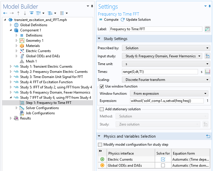
We start with a known signal that has already been converted from the time domain to the frequency domain via the FFT. We will use the IFFT to convert back to the time domain. Starting with the example developed in a previous article, where an FFT of a trapezoidal pulse is taken, the screenshot below shows the Frequency to Time FFT study step that will convert the frequency-domain data back to the time domain.

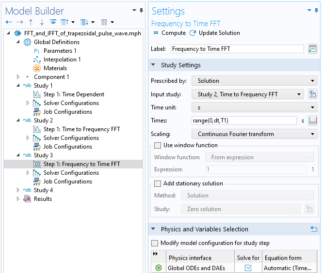
The Model Builder with the Frequency to Time FFT study step selected and the corresponding Settings window.
Screenshot of the Frequency to Time FFT study step settings.

The results of the IFFT are shown below. We have zoomed in to one section, making it possible to see the Gibb's phenomena.

A line graph showing the IFFT results, with one corner of a peak zoomed in to show the Gibb's phenomena.
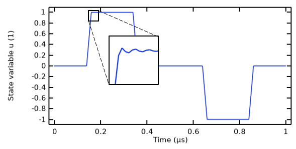
The results of taking an IFFT on the FFT of a trapezoidal pulse.

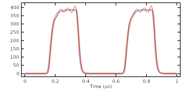
It is also interesting to see how the IFFT reconstructs the signal in terms of the number of harmonics considered. We already know from looking at the FFT that only the odd harmonics carry significant information, and we would like to see what the IFFT looks like by considering only the lowest few harmonics in the IFFT. This is done by using the Window function capability, which can be used to operate on the frequency-domain data, where the frequency is the built-in variable, freq. The screenshot below shows a Boolean expression being used (freq<N*f1), which evaluates to zero or one. It filters out all signals greater than N*f1, where N is a positive integer parameter that is being swept over via the Parametric Sweep feature.

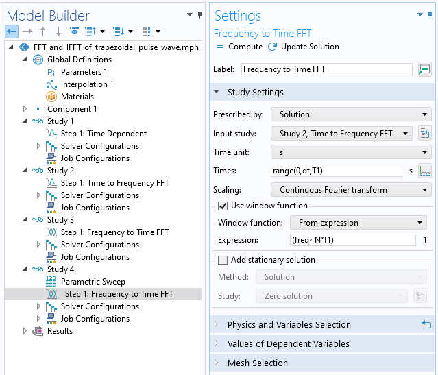
The Model Builder with the Frequency to Time FFT study step selected and the corresponding Settings window with the Use window function check box selected.
Screenshot of the Frequency to Time FFT study step, with the window function being used. The Parametric Sweep is used to sweep over the number of harmonics used in the reconstruction.

The results below show how including an increasing number of harmonics will improve the reconstruction of the original signal.

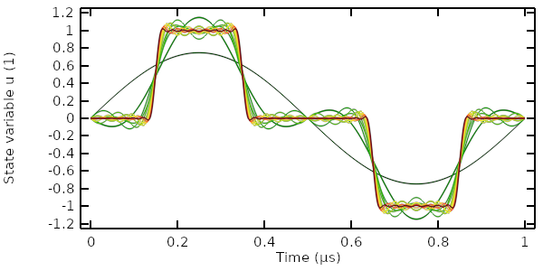
A line graph showing the increasing number of harmonics over time.
The results of taking an IFFT on the FFT of a trapezoidal pulse, with increasing number of harmonics being considered.

We now see how a signal can be converted from the time domain to the frequency domain and back again via the FFT and IFFT. Next, we will look at how the FFT of this signal can be combined with a model of a system to compute the transient response of a model via the IFFT.

Using the IFFT to Reconstruct the Transient Response of a System

Here, we examine a system composed of a coaxial probe inserted into a metal cavity that is filled with a lossy dielectric, with relative permittivity of 50 and electric conductivity of 30 mS/m. The insulator within and surrounding the coax has a relative permittivity of 1.75 and electric conductivity of 1-e12 S/m. The outer conductor of the coax is electrically connected to the cavity walls, and the inner conductor is fed with a time-varying current source. This type of model can be solved with the transient Electric Currents interface since the magnetic fields are negligible.

A cylinder metallic cavity model outlined in yellow, with a coaxial probe inside as well as blue lossy dielectric material.
A model of a coaxial probe inside of a metallic cavity filled with a sample of lossy dielectric material.

Solving this model for one period of the same trapezoidal pulse shown earlier, we can plot the voltage and current at the terminal as well as the losses within the sample. The response shows the typical behavior of a resistive–capacitive system.

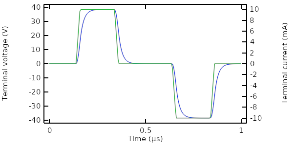
A graph showing the terminal voltage and applied current, with both lines having a peak before 0.5 microseconds and a drop after 0.5 microseconds.
The terminal voltage (blue) and applied current (green) as computed in time.

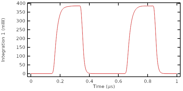
The losses computed over time shown via a red line, which has two peaks over time.
The losses within the sample material computed over time.

We want to reconstruct these results by instead solving the model in the frequency domain, followed by using the FFT of the excitation function that was computed earlier. Begin by solving the model in the frequency domain (using a unit excitation) over a set of harmonics. For this example, we solve for the first 100 harmonics. We then combine the frequency-domain response of the model with the FFT of this input signal via the Window function in the Frequency to Time FFT study, as shown in the screenshot below. The withsol() operator is used to refer to the results of taking the FFT of the excitation function.

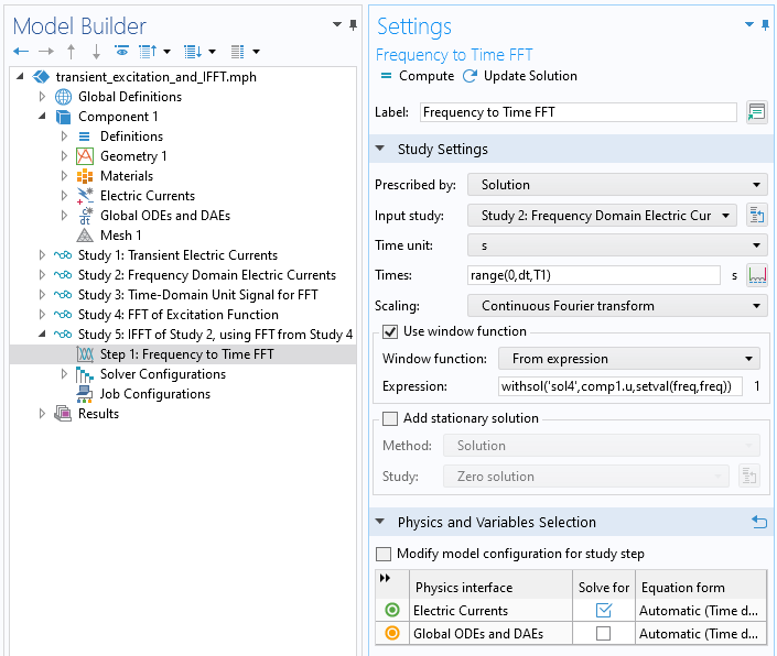
The Model Builder with the Frequency to Time FFT study step highlighted and the corresponding Settings window showing the Input study feature.
Using the Frequency to Time FFT study to take an input study and an FFT as computed from a Time to Frequency FFT study.

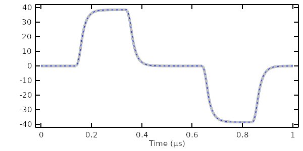
A graph with a thick gray line to show the terminal voltage computed in the time domain, with a dashed blue line overlapping it.
Comparison of terminal voltage computed in the time domain (gray line) versus computed via frequency domain and IFFT (dashed blue line).

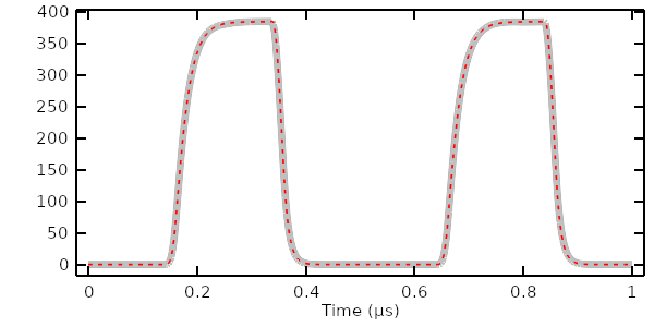
A line graph showing a thick gray line with a red dashed line overlapping it, with both lines having two peaks.
Comparison of losses computed in the time domain (gray line) versus computed via frequency domain and IFFT (dashed red line).

The results show excellent agreement between the transient solution and the solution computed via the IFFT, using the first 100 harmonics.

It is also possible to reconstruct the signal with a smaller subset of nonuniformly spaced harmonics. To see why this is useful, look at the magnitude of the Fourier coefficients of the first 20 harmonics. Observe that all even harmonics are negligible and that the 5^th and 15^th harmonic are also negligible. It is thus justified to solve the frequency-domain model over only a much smaller and nonuniform frequency range.

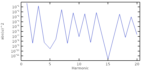
A line graph showing the magnitude of the harmonics, with the blue line having seven sharp peaks.
Magnitude of the Fourier coefficients of the first 20 harmonics of the trapezoidal pulse. Only some of these are significant.

To solve the model, we solve a second Frequency Domain study over a fewer number of harmonics, which will take much less time. Within the Frequency to Time FFT study, we instead have to use the Discrete Fourier transform scaling option rather than the option for continuous scaling. The results show that the terminal voltage and losses in the sample still agree reasonably well.

The COMSOL Multiphysics UI showing the Model Builder with the Frequency to Time FFT study selected and the corresponding Settings window with the Scaling option set to Discrete Fourier transform.
Using the Frequency to Time FFT study with a nonuniform set of frequency-domain results requires the discrete Fourier transform scaling.

A graph showing a thick gray line with a blue line overlapping it, where both lines have one peak around 0.2 microseconds and a drop around 0.7 microseconds."
The terminal voltage computed in the time domain (gray) versus computed via IFFT with only a few harmonics (blue).

A graph showing a thick gray line with a red line overlapping it, where both lines have peaks around 0.2 microseconds and 0.7 microseconds.
The losses computed in the time domain (gray) versus computed via IFFT with only a few harmonics (red).

Extracting Time-Integrated Quantities

It is also useful to extract the total energy deposited into the sample per pulse. This data can be extracted directly from the Time Dependent study results by using the time integration operator:

timeint(0, T1/2, intopSample(ec.Qh), 'nointerp'). This expression integrates without interpolation over only one-half the period since we know already that the signal repeats over the second half of the period and that the integral over the entire period will be twice as much.

The same information can be extracted by combining the frequency-domain solution and the FFT of the input signal via the withsol() operator. The energy dissipated within the sample material, for the N^th harmonic, can be computed via the expression

withsol('sol2',0.5*intopSample(ec.Qh)*T1,setind(freq,N))*withsol('sol4',abs(comp1.u)^2,setind(freq,N+1))

The parameter N is a positive integer. The first withsol operator within this expression uses the frequency-domain results with a factor of one-half applied to the losses for only one pulse, and the setind argument sets the frequency index to the N^th harmonic. The scond withsol operator uses the FFT results, and the setind argument refers to the N+1 solution since the FFT dataset contains the DC solution.

It is possible to plot this data by introducing another Global ODEs and DAEs interface that stores the results of the above evaluation and to solve that within a study that sweeps over a number of harmonics. The results show that for this case over 75% of the dissipation of energy is in the 1^st harmonic; over 95% is in the 1^st and 3^rd; and over 99% is in the 1^st, 3^rd, 7^th, and 9^th. These observations of the system can be very useful when dealing with electromagnetic heating models.

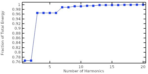
$A graph showing the number of harmonics and fraction of total energy via a blue line, which has a peak before 5 harmonics and then has a slight raise until 20 harmonics.$
The fraction of the total dissipated energy in the system, summed over the first 20 harmonics.

Further Learning

You can open and review the model example shown throughout this article via the downloadable files on this page.

Submit feedback about this page or contact support here.