Understanding Periodic Signals and Their Frequency Content
In this article, we will discuss different types of periodic signals and show how to compute their frequency content in the COMSOL® software.
Introduction
To build up an understanding of the modeling of periodic signals, it is helpful to begin with some simple signals and understand them in terms of their frequency content, as computed via the fast Fourier transform (FFT). Here, we refer to signals in the context of the excitation of an electrical system, so the signal can represent either the current, electric field, or electric potential (voltage) applied to the system over time.
Understanding Simple Signals
The simplest periodic signal is a constant, or DC, signal:  , which is periodic over any time period.
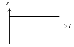
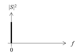
This DC signal has no variation in time, so it has no frequency content. It does carry power, though, at a frequency of zero. If we plot the magnitude of the power carried by the signal as a function of frequency, it will look like:
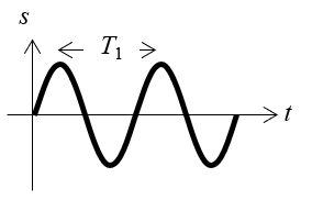
The next simplest signal is a pure sine wave:  , which is an AC signal with period
  .
.
This signal has single-frequency content, so in terms of frequency, its power will look like:
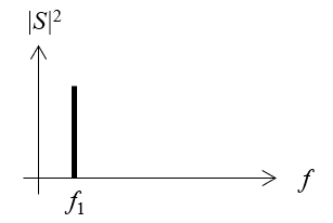
It is important to remark that the plot above is showing the square of the magnitude of a complex-valued number since:

So, the Fourier coefficient of the sine wave is  . Rather than examining the complex-valued coefficients, we are generally more interested in the square of the magnitude,
  , of these coefficients since this is proportional to the power carried by the signal.
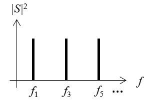
We then consider the extreme of a signal with period  that has infinite frequency content:
  , or the sum of all of the odd harmonics of a sine wave. In the frequency domain, this would look like:
If we plot an approximation of this signal in the time domain, it will approach a pulse that goes to positive and negative infinity, with each pulse having zero duration.
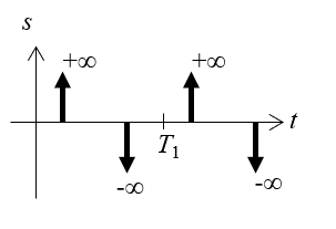
This signal is primarily interesting from a theoretical point of view, as there are no physical devices that can produce such a signal. All real sources will have some maximum frequency content or some finite duration to the pulses. We will choose a signal that lies between these extremes of single-frequency and infinite-frequency content and examine it in more detail.
Understanding the Trapezoidal Pulse Wave
The signal we will examine in detail is the trapezoidal pulse wave, as plotted below.
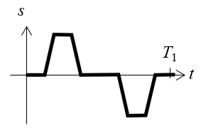
This signal averages to zero over one period, meaning that it has no DC component, that is, no zero-frequency content. It has a fundamental frequency based on the period and a maximum frequency content that depends on both the width of the pulse and the rise/fall time.
It is also worth discussing the periodic trapezoidal pulse train, which is a similar function. It appears as:
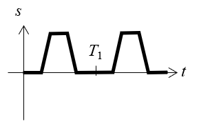
This function looks very similar. It is a strictly positive version of the previous signal. It does not average to zero over one period, so it does have a DC component. However, if we are analyzing these two signals in terms of their effect on a physical system, such as how an applied electric current signal will heat up a material, we can apply some physical insight: If we are dealing with an electrically linear material, then the heat generated by these two signals will be identical. Cases where the assumption of linear materials does not hold include:
- Semiconductors and semiconductor devices, such as diodes
- Electrochemical behavior, such as surface corrosion
- Dielectric breakdown due to, for example, lightning strikes
For most other cases it is sufficient to assume that materials are linear, meaning that they have approximately constant electrical properties, at least over some timespan much longer than the period of the signal. So, comparing the periodic trapezoidal pulse train and the trapezoidal pulse wave shown above, these two functions will lead to the same heating profile over time. Even though the true applied signal might actually be similar to the pulse train in that it is strictly positive, it can be helpful to instead consider a signal that oscillates about zero. This has the advantage that the DC component will be zero, which simplifies the analysis.
Finally, it is worth remarking on the applied signal as it rises and falls. In any real system there will be some smoothing and possibly some oscillatory overshoots and undershoots, as pictured.
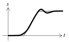
The slope, the smoothing, and the overshoots and undershoots can all contribute to the frequency content in the signal, and it is important to know this as one of the preliminary steps in the modeling process. This example will consider a function without any undershoots and overshoots or smoothing, but the workflow will be the same, even as more complicated functions are used.
Using the FFT to Compute Frequency Content
There are three steps involved in computing the FFT of an arbitrary periodic function:
- Defining the periodic function, over a timespan of one period
- Generating time-domain data over one period, at sufficient resolution for the highest frequency of interest
- Computing the FFT
There are a number of built-in functions in COMSOL Multiphysics® that can be used to define a signal over time. The Piecewise function can be used to define different functions over different intervals and can use any of the mathematical functions. Several of these built-in functions also include smoothing options. It is also possible to use the Interpolation function to read in time-series data from an external text file. The screenshot below shows an example of setting up an unsmoothed trapezoidal pulse wave.
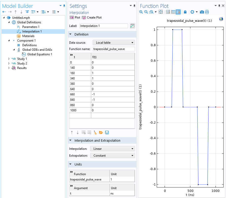
An unsmoothed trapezoidal pulse wave of period 1 µs. The interpolation is set to linear, and the units of the input and function are set.
Next, we need to generate time-domain data over one period. This data has to be at sufficient resolution to resolve the highest frequency that we are interested in. The highest frequency should be defined in terms of an integer multiple of the fundamental, so  . To fulfill the Nyquist criterion, there must be at least two points per period:
  . If we define
  , then we resolve at frequencies up to
  . This also fulfills the condition that there are an even number of time steps used as input to the FFT step.
We do not usually know what the highest frequency content of the signal is ahead of time, so start by resolving a very high maximum frequency. Using the period of our signal, we can arrive at an estimate of the maximum frequency and use it to define a set of parameters that will be used in the FFT study. Start with a very high resolution, check the results, and then recompute with a lower maximum frequency to save computational costs. In the example here, start with a maximum frequency of one thousand times the fundamental.
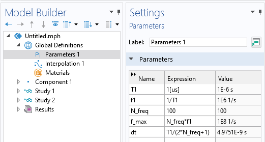
Setting up parameters in preparation for an FFT study. Based on the desired maximum resolved frequency, a time step is chosen that exceeds the Nyquist criterion.
Next, we need to define a dataset in time. This can be done by introducing a variable, u, that has a unit value over the entire period. The screenshot below shows how to set up such a variable.
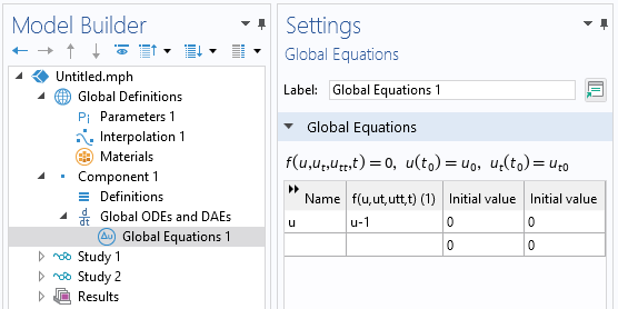
Setting up a global equation for a variable that will be equal to one.
Next, set up a study that will generate a result dataset for one period, with output times based on the Nyquist criterion, as shown in the screenshot below.
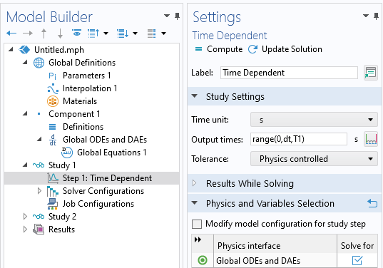
Setting up a time-dependent study that will generate a unit signal in the time domain.
The result of this study will be a dataset that stores the value u = 1, for all time, at the set of time steps that fulfill the Nyquist criterion for the highest frequency of interest. This signal is used within a Time to Frequency FFT study step, along with a window function. The window function is applied to the signal, and since the input signal is one for all time, entering a window function means that we will take the FFT of the window function itself. The screenshot below shows how this is set up to use the results of the previous study. Note that it is possible to set up multiple studies that will take the FFT of different window functions.
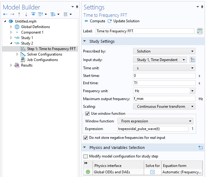
Using the Time to Frequency FFT study, with the Window function feature, to take the FFT of a trapezoidal pulse wave.
After running this study, the related dataset for u will contain the FFT of the window function, and this will be a complex-valued number corresponding to the Fourier coefficient for the range of frequencies:  . Note that this includes the zero frequency, or DC component, of the signal, which we know will be zero.
In terms of understanding the frequency content, it is primarily useful to think in terms of the power, or energy, in the signal, which is proportional to the square magnitude of the coefficients. So, we plot the expression abs(u)^2, which represents the power in the signal. The results of the FFT will look similar to the plot below.
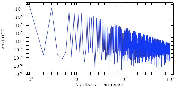
Plot of the power in a trapezoidal pulse wave versus frequency, starting with the fundamental frequency.
From this plot, which is in log–log scale, we can observe a few things. First, for this signal, only the odd harmonics, , contribute very much. Second, the very high frequency content from 100–1000 times the fundamental is negligible. We are thus justified in reducing the computation by rerunning the FFT to consider only the first 100 harmonics. This will be important in the next step, when we reconstruct the time-domain behavior of a real system by first solving in the frequency domain over a smaller set of frequencies, and then use the inverse FFT to reconstruct an approximation of the time-domain solution. To continue with the next step, refer to Using the Inverse Fast Fourier Transform to Reconstruct a Transient Signal.
It can also be useful to plot out the summed fraction of the power content in the signal, which involves summing up the square of the magnitude of the coefficients over the number of harmonics. This can be done via a combination of the sum() and with() operators:
sum(with(ind+1,abs(u)^2),ind,0,freq/f1)/sum(with(ind+1,abs(u)^2),ind,0,f_max/f1)
The with() operator will refer to an indexed number from the current solution. The sum() operator defines an index that goes from the specified lower limit to upper limit. Note that the sum starts from index zero, the 0th harmonic, or the DC component, even though we know that this is zero for this case. The expression shown above will thus sum up the square of the magnitude of the Fourier coefficients. This expression can be used to plot the sum over a number of harmonics, as shown below for the first 100 harmonics.
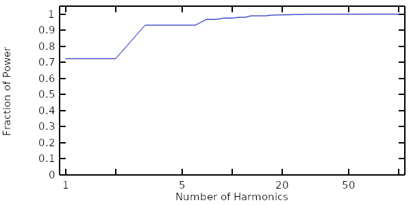
Plot of the cumulative power in the signal summed over a number of harmonics.
Further Learning
The model example shown in this article is available for download from the sidebar to the right. As mentioned earlier, a good next step after exploring this model is to check out Using the Inverse Fast Fourier Transform to Reconstruct a Transient Signal.
Furthermore, there is additional information on the types of functions you can use to define periodic signals, as well as how to define them, in the COMSOL Multiphysics documentation linked below:
Submit feedback about this page or contact support here.