Learning Center

BACK TO LEARNING CENTER

Modeling Capacitive Discharge

Here, we address how to model the discharging of a capacitor that is connected to a set of electrical components, which can be modeled either with full geometric fidelity or in combination with a set of lumped components.

Background

It is possible to model the discharge of the electric energy stored within a capacitor using the Electromagnetic Waves, Transient interface. The initial stored electric energy can either be computed using the Electrostatics interface, which solves for the electric fields within the structure of the capacitor, or alternatively, the capacitor can be modeled using the Electrical Circuits interface, where a lumped capacitor with an initial charge defines the initial stored electric energy. The objective of these models is to compute the electromagnetic fields and the losses. The electric and magnetic energy are computed, as well as the conversion into thermal energy and the radiated energy.

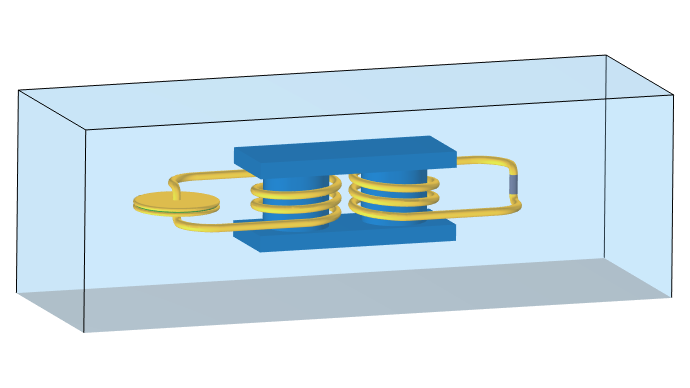
A capacitor model connected to electrical components surrounded by free space.

The structure being modeled. An explicitly modeled capacitor is connected to a transformer, which is then connected to a Lumped Element model of a capacitor equivalent. Supporting structures are omitted under the assumption that they are not electromagnetically relevant. The surrounding region of free space and a ground plane are modeled.

Modeling Approach

Discharge modeling involves two steps: first, setting up an electrostatics model that computes the electric fields around a charged capacitor and then using those fields as initial conditions in a transient electromagnetic model. You can follow along using the MPH-file attached to this article.

The Electrostatics Model

To model the initial charge, the modeling domain is partitioned to consider only the dielectric and a small volume of space around the capacitor where there will be significant electric fields. Within this domain, the boundary conditions are set to Ground on one of the capacitor plates, and a fixed Electric Potential on the other plate. The interior of the connecting wires is not modeled. All other boundaries are set to Zero Charge. The solution from this electrostatic model is used as the initial state for the transient electromagnetic problem, where the wires will be explicitly modeled.

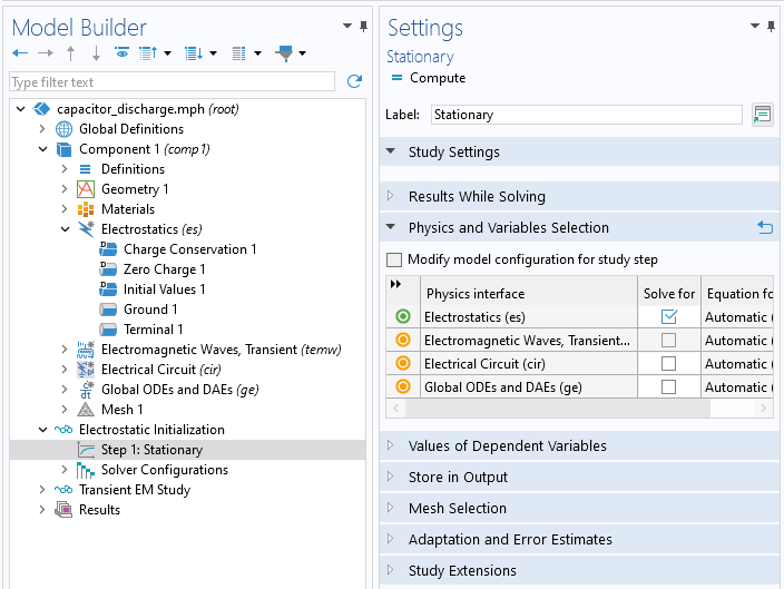A close-up view of the Model Builder with the Stationary node highlighted and the corresponding Settings window.

A separate Stationary study is used to solve for the electrostatic fields in the dielectrics around the capacitor plates. Within this study, only the Electrostatics interface is solved for.

The Transient Electromagnetic Model

To model the transient behavior, the Electromagnetic Waves, Transient interface is solved on all domains with the exception of a domain representing the lumped Electrical Circuit elements. This cylindrical domain bridges a gap in the conductive wires. The Electrical Circuit adds additional impedance to the system across this gap and is connected via the Lumped Port feature, of type Via. The Lumped Port feature is valid to use under the assumption that the electric field is uniform and parallel to the wire around its perimeter. The cross-sectional boundaries of the wire on either end of the Via are Perfect Electric Conductor, implying an equipotential condition across these surfaces.

The Perfect Electric Conductor boundary condition is applied on the bottom boundary of the model, representing a lossless ground plane. The remaining outside boundaries of the domain are Scattering Boundary Conditions, which approximate an open boundary to free space. Electromagnetic waves will pass through these boundaries with minimal reflections.

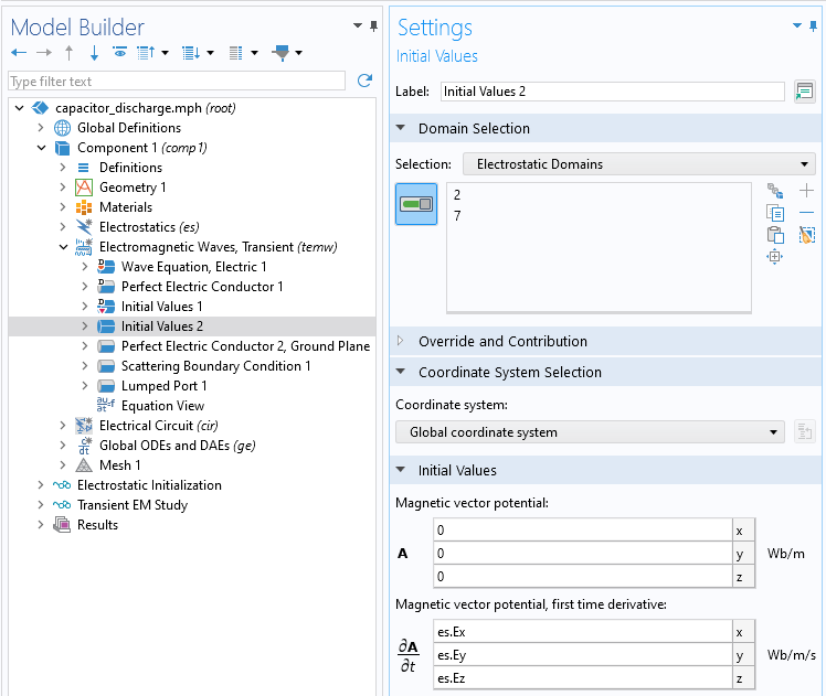
The Initial Values feature defines the computed electrostatic fields as the initial value for the first time derivative of the Magnetic vector potential field.

A close-up view of the Model Builder with the Time Dependent node highlighted and the corresponding Settings window.

The study is set up to first solve for the initial electrostatic fields, then compute the electromagnetic fields, the lumped circuit, and a set of global equations for the power and energy. The initial values used to compute the electromagnetic fields are taken from the electrostatic initialization. It is also possible to save results only on some selections to reduce the amount of data stored.

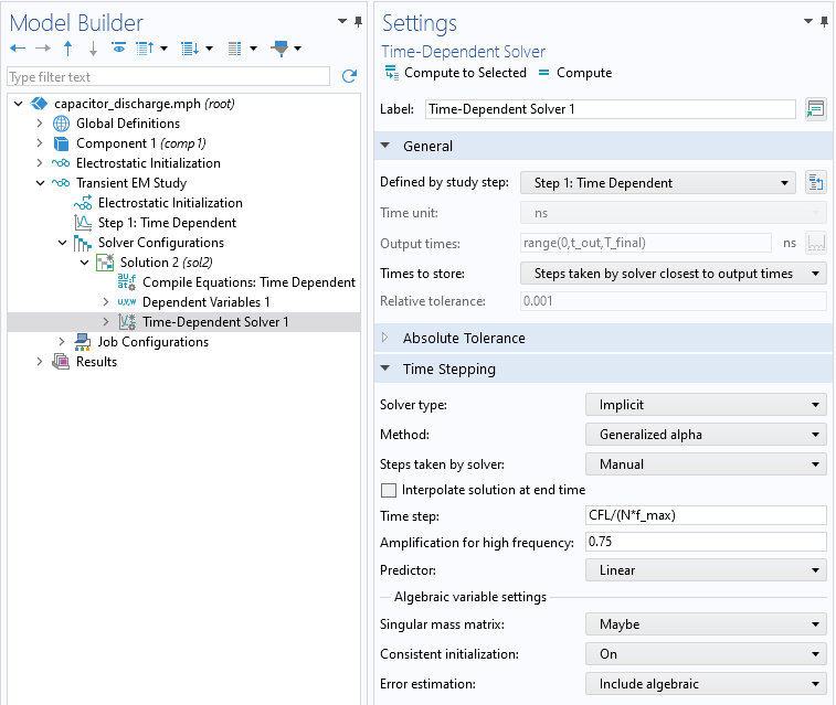A close-up view of the Model Builder with the Time-Dependent Solver node highlighted and the corresponding Settings window.

The Time-Dependent Solver settings are adjusted based on the maximum frequency of interest and the element size. Consistent initialization is on.

A Time Dependent study is used to solve for the electromagnetic fields over time. Based on the maximum frequency of interest, it is possible to manually specify the time step, which reduces the computational cost. Since the global equations are used to store all integrated quantities, it is possible to reduce the amount of data that is stored in the model by only saving results on a few selected domains, or none at all.

Results and Discussion

It is useful to examine the plot of energy as well as the relative losses. Note that:

The total energy of the system is nearly constant over time. In the limit of mesh and time-step refinement, this can be improved further.
The frequency content is initially high but reduces over time.
The fraction of total thermal losses in the conductors is relatively small. It is possible to ignore losses in the conductors altogether by omitting these domains from the analysis and modeling the boundaries of the conductors as Perfect Electric Conductor boundary conditions.
The model can instead be run with the lumped capacitor having an initial potential, and discharging into the modeled domains.

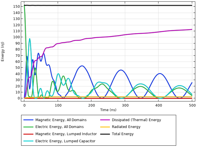A 1D plot showing the magnetic, electric, dissipated, radiated, and total energy over time.

Plot of the electric, magnetic, thermal, and radiated energy over time. The sum stays nearly constant.

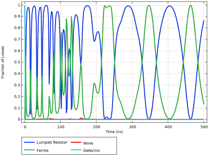A 1D plot showing the total thermal losses over time.

The thermal losses as a fraction of total losses.

Further Learning

To learn more about the techniques introduced here and explore new ones, check out the following resources:

Submit feedback about this page or contact support here.