

In Part 2 of our blog series on multiscale modeling in high-frequency electromagnetics, we discuss a practical implementation of multiscale techniques in the COMSOL Multiphysics® software. We will simulate radiated fields using two different techniques and verify our results with theory. While these methods can be generally applied, we will always revolve around the practical issue of antenna-to-antenna communication. For a review of the theory and terms, you can refer to the first post in the series.
Simulating a Radiating Antenna
Let’s begin by discussing a traditional antenna simulation using COMSOL Multiphysics and the RF Module. When we simulate a radiating antenna, we have a local source and are interested in the subsequent electromagnetic fields, both nearby and outgoing from the antenna. This is fundamentally what an antenna does. It converts local information (e.g., voltage or current) into propagating information (e.g., outgoing radiation). A receiving antenna inverts this operation and changes incident radiation into local information. Many devices, such as a cellphone, act as both receiving and emitting antennas, which is what enables you to make a phone call or browse the web.
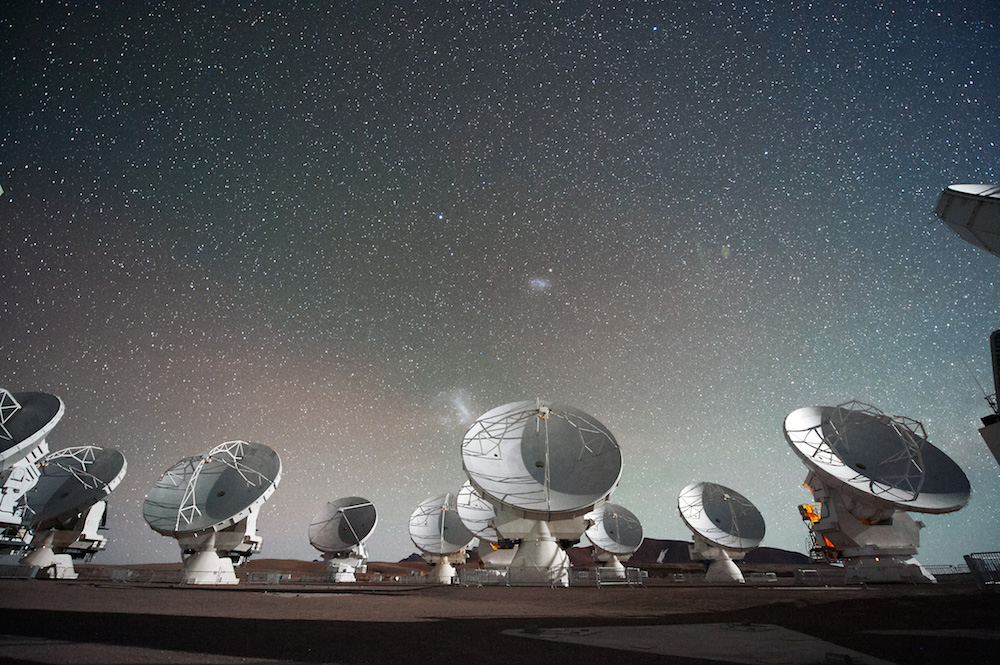
Antennas of the Atacama Large Millimeter Array (ALMA) in Chile. ALMA detects signals from space to help scientists study the formation of stars, planets, and galaxies. Needless to say, the distance these signals travel is much greater than the size of an antenna. Image licensed under CC BY 4.0, via ESO/C. Malin.
In order to keep the required computational resources reasonable, we model only a small region of space around the antenna. We then truncate this small simulation domain with an absorbing boundary, such as a perfectly matched layer (PML), which absorbs the outgoing radiation. Since this will solve for the complex electric field everywhere in our simulation domain, we will refer to this as a Full-Wave simulation.
We then extract information about the antenna’s emission pattern using a Far-Field Domain node, which performs a near-to-far-field transformation. This approach gives us information about the electromagnetic field in two regions: the fields in the immediate vicinity of the antenna, which are computed directly, and the fields far away, which are calculated using the Far-Field Domain node. This is demonstrated in a number of RF models in the Application Gallery, such as the Dipole Antenna tutorial model, so we will not comment further on the practical implementation here.
Using the Far-Field Domain Node
One question that occasionally comes up in technical support is: “How do I use the Far-Field Domain node to calculate the radiated field at a specific location?” This is an excellent question. As stated in the RF Module User’s Guide, the Far-Field Domain node calculates the scattering amplitude, and so determining the complex field at a specific location requires a modification for distance and phase. The expression for the x-component of the electric field in the far field is:
and similar expressions apply to the y– and z-component, where r is the radial distance in spherical coordinates, k is the wave vector for the medium, and emw.Efarx is the scattering amplitude. It is worth pointing out that emw.Efarx is the scattering amplitude in a particular direction, and so it depends on angular position (\theta, \phi), but not radial position. The decrease in field strength is solely governed by the 1/r term. There are also variables emw.Efarphi and emw.Efartheta, which are for the scattering amplitude in spherical coordinates.
To verify this result, we simulate a perfect electric dipole and compare the simulation results with the analytical solution, which we covered in the previous blog post. As we stated in that post, we split the full results into two terms, which we call the near- and far-field terms. We briefly restate those results here.
\overrightarrow{E} & = \overrightarrow{E}_{FF} + \overrightarrow{E}_{NF}\\
\overrightarrow{E}_{FF} & = \frac{1}{4\pi\epsilon_0}k^2(\hat{r}\times\vec{p})\times\hat{r}\frac{e^{-jkr}}{r}\\
\overrightarrow{E}_{NF} & = \frac{1}{4\pi\epsilon_0}[3\hat{r}(\hat{r}\cdot\vec{p})-\vec{p}](\frac{1}{r^3}+\frac{jk}{r^2})e^{-jkr}
\end{align}
where \vec{p} is the dipole moment of the radiation source and \hat{r} is the unit vector in spherical coordinates.
Below, we can see the electric fields vs. distance calculated using the Far-Field Domain node for a dipole at the origin with \vec{p}=\left(0,0,1\right)A\cdot m. For comparison, we have included the Far-Field Domain node, the full theory, as well as the near- and far-field terms individually. The fields are evaluated along an arbitrary cut line. As you can see, there is overlap between the Far-Field Domain node and the far-field theory plots, and they agree with the full theory as the distance from the antenna increases. This is because the Far-Field Domain node will only account for radiation that goes like 1/r, and so the agreement improves with increasing distance as the contribution of the 1/r2 and 1/r3 terms go to zero. In other words, the Far-Field Domain node is correct in the far field, which you probably would have guessed from the name.
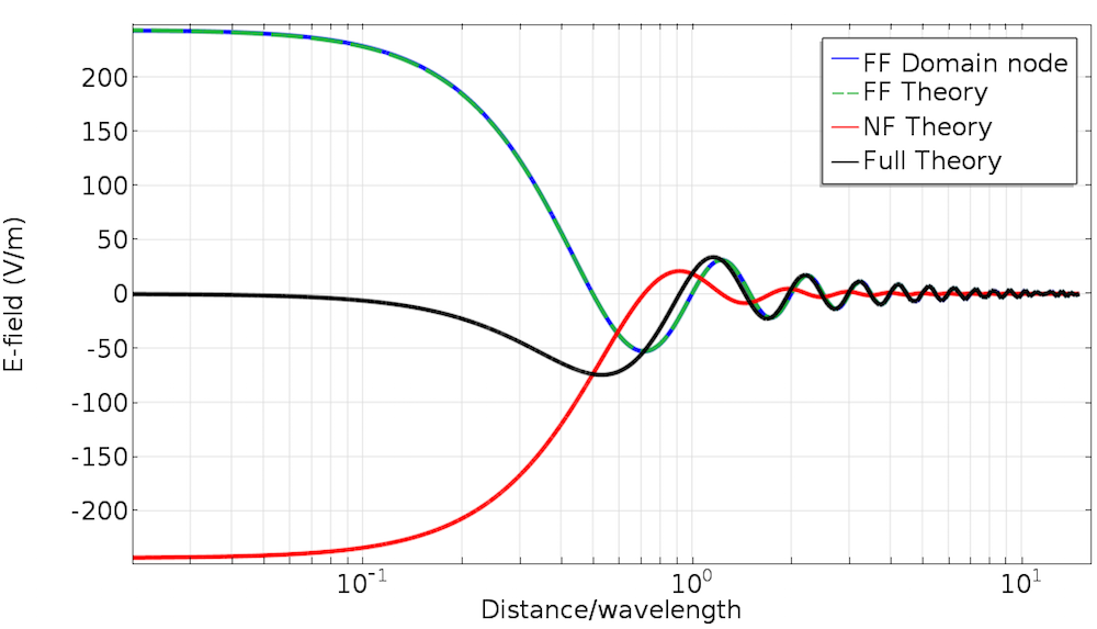
A comparison of the Far-Field Domain node vs. theory for a point dipole source.
Using the Electromagnetic Waves, Beam Envelopes Interface
For most simulations, the near-field and far-field information is sufficient and no further work is necessary. In some cases, however, we also want to know the fields in the intermediate region, also known as the induction or transition zone. One option is to simply increase the simulation size until you explicitly calculate this information as part of the simulation. The drawback of this technique is that the increased simulation size requires more computational resources. We recommend a maximum mesh element size of \lambda/5 for 3D electromagnetic simulations. As the simulation size increases, the number of mesh elements increases, and so do the computational requirements.
Another option is to use the Electromagnetic Waves, Beam Envelopes interface, which here we will simply refer to as Beam-Envelopes. As discussed in a previous blog post, Beam-Envelopes is an excellent choice when the simulation solution will have either one or two directions of propagation, and will allow us to use a much coarser mesh. Since the phase of the emission from an antenna will look like an outgoing spherical wave, this is a perfect solution for determining these fields. We perform a Full-Wave simulation of the fields near the source, as before, and then use Beam-Envelopes to simulate the fields out to an arbitrary distance, as required.
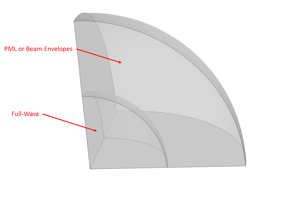
The simulation domain assignments. If the outer region is assigned to PML, then a Full-Wave simulation is performed everywhere. It is also possible to solve the inner region using a Full-Wave simulation and the outer region using Beam-Envelopes, as we will discuss below. Note that this image is not to scale, and we have only modeled 1/8 of the spherical domain due to symmetry.
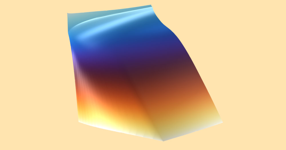
How do we couple the Beam-Envelopes simulation to our Full-Wave simulation of the dipole? This can be done in two steps involving the boundary conditions at the interface between the Full-Wave and Beam-Envelopes domains. First, we set the exterior boundary of the Full-Wave simulation to PMC, which is the natural boundary condition for that simulation. The second step is to set that same boundary to an Electric Field boundary condition for Beam-Envelopes. We then specify the field values in the Beam-Envelopes Electric Field boundary condition according to the fields computed from the Full-Wave simulation, as shown here.
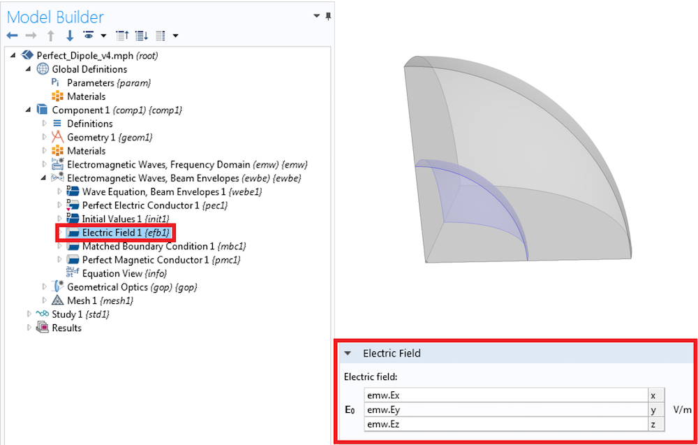
The Electric Field boundary condition in Beam-Envelopes. Note that the image in the top right is not to scale.
A Matched Boundary Condition is applied to the exterior boundary of the Beam-Envelopes domain to absorb the outgoing spherical wave. The remaining boundaries are set to PEC and PMC according to symmetry. We must also set the solver to Fully Coupled, which is described in more detail in two blog posts on solving multiphysics models and improving convergence from a previous blog series on solvers.
If we again examine the comparison between simulation and theory, we see excellent agreement over the entire simulation range. This shows that the PMC and Electric Field boundary conditions have enforced continuity between the two interfaces and they have fully reproduced the analytical solution. You can download the model file in the Application Gallery.
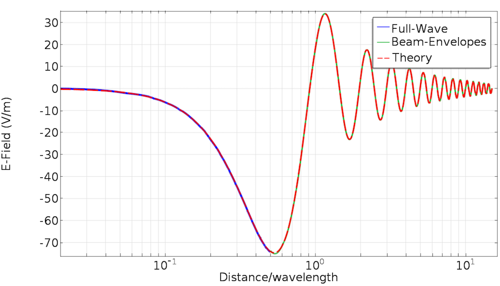
A comparison of the electric field of the Full-Wave and Beam-Envelopes simulations vs. the full theory.
Concluding Thoughts on Simulating a Radiating Source in COMSOL Multiphysics®
In today’s blog post, we examined two ways of computing the electric field at points far away from the source antenna and verified the results using the analytical solution for an electric point dipole. These two techniques are using the Far-Field Domain node from a Full-Wave simulation and linking a Full-Wave simulation to a Beam-Envelopes simulation. In both cases, the fields near the source and in the far field are correctly computed. The coupled approach using Beam-Envelopes has the additional advantage in that it also computes fields in the intermediate region. In the next post in the series, we will combine the calculated far-field radiation with a simulation of a receiving antenna and determine the received power. Stay tuned!
Read the Full Series
- Browse the other posts in the Multiscale Modeling for High-Frequency Electromagnetics blog series


Comments (6)
Robert Koslover
January 16, 2017Thank you for this article. See https://www.comsol.com/community/exchange/247/
for an alternative approach; I would be interested in your thoughts about it.
Linus Andersson
January 20, 2017Hi Robert, that’s great! I had thought this would be possible; I just hadn’t seen anyone implement it in an Electromagnetic Waves interface before. We do have a similar general formulation (“Full integral”) in Pressure Acoustics.
Mamad Moka
August 20, 2017this BLOG can be very useful
Mamad Moka
August 27, 2017why the exterior boundary of electromagnetic fullwave (emw) is set to perfect magnetic conductor ?is it a general rule(for example can I perform this boundary condition for horn antenna )? I think this boundary condition will affect near field of small dipole antenna.
Linus Andersson
September 12, 2017Hi Mamad, you should only use the natural condition (in this case Perfect Magnetic Conductor) for continuity when you are connecting two interfaces across a common boundary. The other interface then needs a Dirichlet condition, such as the Electric Field condition used here. On an exterior boundary with no coupling to another interface, the Perfect Magnetic Conductor condition would indeed reflect the field.
Robert Koslover
January 6, 2019My paper linked above was accidentally deleted, but it has been re-posted. It can be found at https://www.comsol.com/community/exchange/672/ .