
Did you know that you can analyze twist and bending in a 2D axisymmetric Solid Mechanics interface? Functionality in the COMSOL Multiphysics® software, as of version 6.0, allows you to easily set up models in 2D axisymmetry, which would normally require a full 3D analysis. Using the extended formulation, you can study, for example, anisotropic materials that twist due to axial forces, circumferential cracks loaded in torsion, or stress concentration factors for bending — all while working with a 2D geometry. Let’s take a look at how it works.
What Is 2D Axisymmetry?
In our previous blog post “What Is the Difference Between Plane Stress and Plane Strain?”, we discussed the analysis of 3D solid objects with plane 2D approximations by making assumptions about the stress or strain field in the out-of-plane direction. 2D axisymmetry is another way to reduce a 3D part to a 2D geometry. Modeling in two dimensions has the advantage of being computationally leaner than building a full 3D model, while also allowing for simpler application of boundary conditions and simpler meshing.
Working in 2D axisymmetry requires the geometry and (usually, but not always) the loads and constraints to be constant around the object’s circumference. If these requirements are fulfilled, it is possible to formulate the equations of motion using only a 2D cross section. The 2D slice is sufficient to recover the full 3D stress state and strain state by integrating the governing equations over the full revolution. Typical candidates for 2D axisymmetric analyses are pressure vessels, loudspeaker modules, fluid mixers, O-rings, or shafts.


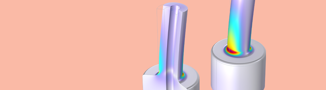
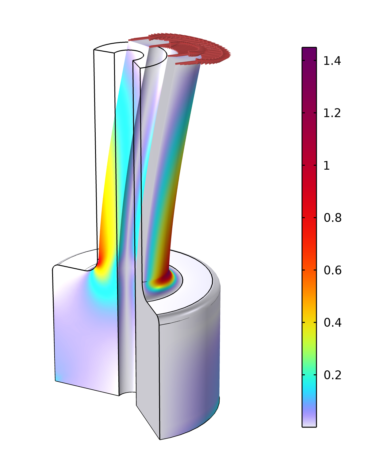
Typical 2D axisymmetric analysis: A 3D shaft (left), its 2D axisymmetric geometry representation with axial load applied at the top (center), and a section of the recovered 3D solution showing a von Mises stress distribution (right).
By default, only the radial and axial displacements, u and w, are solved for in 2D axisymmetry. The circumferential component, v, is assumed to be zero. However, it is possible to include the circumferential displacement, v, which allows twisting deformations in 2D axisymmetry. To get a better understanding of how the extension works, let’s first recap how deformations are generally described using the displacement gradient. Feel free to skip the next section if you are familiar with its concept.
The Displacement Gradient
The Solid Mechanics interface solves the equations of motion, or Newton’s second law. The Equation section in the default Linear Elastic Material node shows the familiar “mass times acceleration equals the sum of all forces” expressed in terms of volume loads, as well as the linear relation between stress and strain, which is the distinct characteristic of this particular material model.
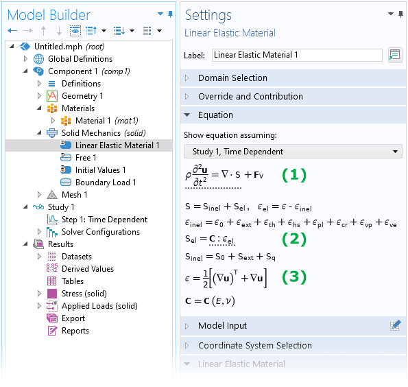
The Equation section of the Linear Elastic Material node shows the equation of motion (1) and the linear elastic constitutive equation (2), as well as the definition of the engineering strain (3).
To formulate a constitutive relation in continuum mechanics analyses, it is necessary to describe the deformation of the material at any given point using some suitable measure. There are in fact numerous measures to choose from when characterizing deformations , such as engineering strain (see (3) in the image above), Green-Lagrange strain, or logarithmic strain, to name a few. The usefulness of these measures depends on the context, such as when using a particular material model or if the model involves large deformations (geometric nonlinearity). However, all of these measures can be expressed as a function of the displacement gradient, \nabla \mathbf{u} (sometimes denoted \textrm{grad} \, \mathbf{u}).
But what is the displacement gradient, and where does it come from? Consider an (infinitesimally) small “blob” of material, which could be part of any larger structure. Initially, at time t_0, the blob has a reference configuration (see the gray surface below). At some later time, t, the blob may have undergone a rigid body motion (translation and rotation) as well as deformations (stretching or shearing), as shown in the animation below.
A plane 2D blob translating, rotating, and deforming elastically (pure shear), visualized as separate deformation steps. The displacement gradient is used to describe the change in displacement between two initially neighboring points, like \textrm{P}_1 and \textrm{P}_2, after the blob has deformed.
In the animation, two points, \textrm{P}_1 and \textrm{P}_2, have been marked. They are assumed to be infinitesimally close to each other. Initially, the point \textrm{P}_1 has the position \mathbf{X}, whereas its current position at time t is denoted \mathbf{x}. The new position of point \textrm{P}_1 may also be described in terms of the original position plus a displacement vector, i.e., \mathbf{x} = \mathbf{X} + \mathbf{u}(\mathbf{X}, t).
Now, let’s focus on the closely neighboring point, \textrm{P}_2. Similar to the first point, \textrm{P}_2 also displaces to a new position after time t. The only difference is that point \textrm{P}_2 is located a small distance away from \textrm{P}_1; that is, its initial position is \mathbf{X} + \textrm{d}\mathbf{X}. Therefore, after the blob has deformed, the new position of \textrm{P}_2 is
This relation can be rearranged slightly to give an expression for \textrm{d}\mathbf{x}, which is the small step between points \textrm{P}_1 and \textrm{P}_2 in the deformed configuration.
= \mathrm{d}\mathbf{X} + \mathrm{d}\mathbf{u} \\[1mm]
Here, the displacement gradient \nabla \mathbf{u} is defined as the tensor, which maps the small step \textrm{d}\mathbf{X} (in the initial configuration) to the change in displacement between points \textrm{P}_1 and \textrm{P}_2 when the body has deformed. The closely related term I + \nabla \mathbf{u} = \textrm{d}\mathbf{x}/\textrm{d}\mathbf{X} is called deformation gradient (often denoted by F), which is a measure that also shows up in many continuum mechanics books.
In more practical terms, \nabla \mathbf{u} is a tensor containing the derivatives of the displacement field \mathbf{u} = (u, v, w)^\textrm{T} with respect to the initial configuration (also material frame coordinates). For a 3D Cartesian system, the displacement gradient is simply
\left[
{\begin{array}{ccc}
\frac{\partial u}{\partial X} & \frac{\partial u}{\partial Y} & \frac{\partial u}{\partial Z} \\
\frac{\partial v}{\partial X} & \frac{\partial v}{\partial Y} & \frac{\partial v}{\partial Z} \\
\frac{\partial w}{\partial X} & \frac{\partial w}{\partial Y} & \frac{\partial w}{\partial Z} \\
\end{array} }
\right]
In 2D axisymmetry, a cylindrical system is used, in which case the displacement gradient is defined as
\left[
{\begin{array}{ccc}
\frac{\partial u}{\partial R} & \frac{1}{R} \frac{\partial u}{\partial \Phi}-\frac{v}{R} & \frac{\partial u}{\partial Z} \\
\frac{\partial v}{\partial R} & \frac{1}{R} \frac{\partial v}{\partial \Phi}+\frac{u}{R} & \frac{\partial v}{\partial Z} \\
\frac{\partial w}{\partial R} & \frac{1}{R} \frac{\partial w}{\partial \Phi} & \frac{\partial w}{\partial Z} \\
\end{array} }
\right]
Here, R, \Phi, and Z are the radial, circumferential, and axial coordinates, respectively.
Adding the Twist…
So, how can the displacement gradient be redefined to extend a simple 2D analysis to what’s sometimes referred to as a 2.5D analysis?
By default, the displacement in the circumferential direction of a 2D axisymmetric solid is assumed to be zero. This is because there are many use cases involving only radial and axial displacements, and adding the displacement component v to the list of dependent variables adds a certain computational cost. Therefore, to study twist in 2D axisymmetry, the circumferential displacement must be added explicitly. This can easily be done using the Include circumferential displacement check box in the Settings window of the Solid Mechanics interface.


The check boxes in the Axial Symmetry Approximation section enable circumferential displacements in 2D axisymmetric models (left). When the Include circumferential displacement check box is selected, many nodes in the Model Builder show additional user inputs, such as fields to apply loads in the azimuthal direction (right).
Selecting the Include circumferential displacement check box does three important things:
- Adds the circumferential displacement component v as a new dependent variable
- Shows new user inputs to, for example, apply loads, springs, or dampers in the circumferential direction
- Modifies the definition of the displacement gradient
The last step allows us to resolve shear strains in the out-of-plane direction (that is, \varepsilon_{R\Phi} and \varepsilon_{\Phi{Z}}), which in typical 2D axisymmetric analyses, are assumed to be zero. The only limitation is that the displacement field must be constant around the object’s circumference. In other words, derivatives with respect to \Phi are assumed to be zero (\partial (…)/\partial \Phi=0). The redefined displacement gradient is therefore
\left[
{\begin{array}{ccc}
\frac{\partial u}{\partial R} & -\frac{v}{R} & \frac{\partial u}{\partial Z} \\
\frac{\partial v}{\partial R} & \frac{u}{R} & \frac{\partial v}{\partial Z} \\
\frac{\partial w}{\partial R} & 0 & \frac{\partial w}{\partial Z} \\
\end{array} }
\right]
where all terms involving v would normally be neglected for standard 2D axisymmetric cases. The extension described here is available for all study types.
Including the circumferential displacement makes it possible to study cases that would normally require a full 3D analysis. Two such examples are shown below. The first example shows a tube made of anisotropic material, such as a fiber composite with an unbalanced layup. In this case, the elasticity matrix contains coupling-terms, which causes the tube to twist when pulled axially. The second example shows a container with a circumferential crack. It is loaded with internal pressure and circumferential forces, which results in the crack being subjected to both opening and out-of-plane shearing modes.
Examples for analyses that typically require full 3D models: normalized circumferential displacement for a tube with a tension-twist coupling due to anisotropic material properties (left), and a von Mises stress distribution for a thick-walled container with a crack loaded in opening and out-of-plane shearing modes (right).
Circumferential Mode Extension
The abovementioned limitation to only allow a constant displacement in \Phi direction can be lifted slightly for eigenfrequency and frequency-domain analyses. For some problems, such as torsional vibrations, it can be reasonable to assume that the solution has a certain periodicity around the circumference. This idea is conveniently expressed with a complex-valued ansatz for the displacement:
This is a valid solution assuming a linear response, which is the most common underlying assumption for frequency-domain analyses anyway. Above, m is the azimuthal mode number defining the number of periods in the displacement field. With this ansatz, the displacement gradient becomes
\begin{bmatrix}
\frac{\partial u}{\partial R}&-\frac{v}{R}& \frac{\partial u}{\partial Z} \\
\frac{\partial v}{\partial R} &\frac{u}{R}& \frac{\partial v}{\partial Z} \\
\frac{\partial w}{\partial R}&0& \frac{\partial w}{\partial Z} \end{bmatrix} – i \frac{m}{R} \begin{bmatrix}
0 & u & 0 \\
0 & v & 0 \\
0 & w & 0
\end{bmatrix}
This type of 2D axisymmetric extension is also referred to as circumferential mode extension, and can be activated with the second check box in the Axial Symmetry Approximation section (see the screenshot above). The mode number must be specified as a user input.
There are two noteworthy special cases:
- m=0, which corresponds to a constant v displacement
- m=1, which can describe bending deformations in 2D axisymmetry
Note that COMSOL Multiphysics automatically modifies the axial symmetry condition (u=v=0) at the symmetry line so that bending deformations are permitted.
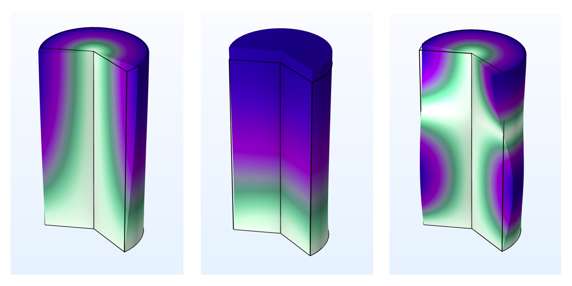
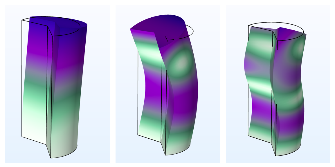
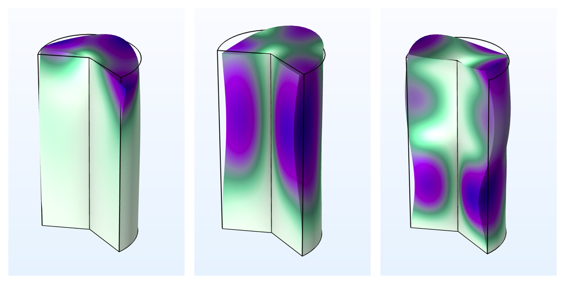
The figure below shows examples of eigenmodes, which can be studied using the circumferential mode extension. By varying the mode number, it is possible to find all of the eigenmodes found in a corresponding, full 3D analysis — provided that the fundamental axisymmetric assumptions hold.
| m=0 |
|
| m=1 |
|
| m=2 |
|
The first three eigenmodes of a cylinder, fixed at one end for different mode numbers, m. In this example, m=0 yields torsional and axial modes, m=1 shows only bending modes, and m=2 displays higher-order torsional modes.
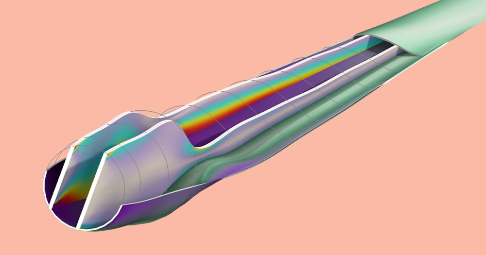
In general, the circumferential mode extension can only be used in eigenfrequency and frequency-domain studies. In stationary and time-dependent studies, the circumferential displacement, v, is kept constant, which corresponds to a mode number m=0. However, if you run a frequency-domain analysis with a frequency of 0\,\textrm{Hz}, you will get a stationary solution since all inertial terms become zero and all loads become frequency independent. Using this trick, it is possible to compute static bending deformations in 2D axisymmetry. The figure below shows an example where a shaft is subjected to bending forces (mode number m=1) and the axial stress, \sigma_z, is compared to the analytically expected stress in the transition region between the thinner and thicker shaft sections.
A shaft subjected to bending forces modeled in 2D axisymmetry. The plot shows the stress concentration factor, or, more precisely, the ratio between the actual stress, \sigma_z, and the expected normal stress in the fillet region, as obtained from elementary bending theory.
A link to this model — including details on how to apply the loads in this case — can be found below.
What About Other Structural Mechanics Interfaces?
The general idea to extend a 2D formulation with an out-of-plane degree of freedom in order to solve for a more intricate displacement field is not unique. The Shell interface, for instance, also supports the circumferential mode extension. And the Plane 2D equivalent in the Solid Mechanics interface is called the Out-of-plane mode extension, and can be enabled in the 2D Solid Mechanics Settings window. It allows users to model wave-like displacements in the out-of-plane direction.
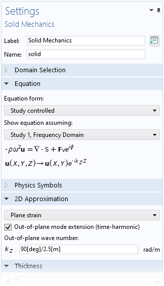
The Out-of-plane mode extension check box for Solid Mechanics with a 2D plane strain formulation.
Also, some other physics interfaces support solving for more advanced 3D fields using similar types of extensions. In fluid interfaces, for instance, the option is called Swirl Flow.
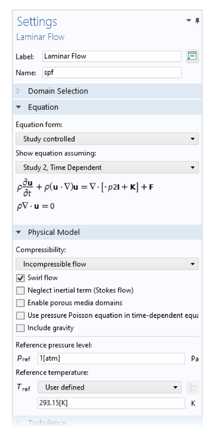
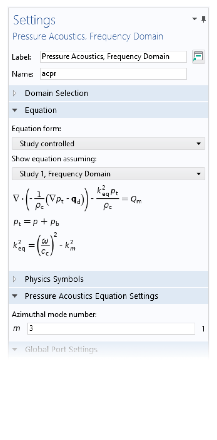
Settings for the 2D axisymmetric Laminar Flow and the Pressure Acoustics, Frequency Domain interfaces. The Swirl Flow and Azimuthal mode number settings allow to solve for more complex-shaped fields around the circumferential direction.
Try It Yourself
Want to try modeling the twist and bending in 2D axisymmetry discussed in this blog post? Click the button below to access the MPH-file.


Comments (0)