

In addition to the general Solid Mechanics interface, the Structural Mechanics Module consists of specialized interfaces: Shell, Plate, and Membrane for the modeling of thin structures; and Beam and Truss for modeling slender structures. An engineering structure that has a mix of solid, thin, and slender components can be modeled by combining these physics interfaces with each other. Here, we will explore the options for coupling the structural mechanics interfaces by using examples from the Model Library.
Structural Mechanics Module Interfaces
First, let us have a look at the interfaces available in the Structural Mechanics Module. The following table lists the interfaces, their space dimension, geometric entity, and the type of structures they are intended for.
| Interface | Space Dimension | Geometric Entity | Type of Structure |
|---|---|---|---|
| Solid Mechanics | 3D, 2D, 2D Axisymmetry | Domain | Any structure |
| Shell | 3D | Boundary | Thin flat or curved structures with significant bending stiffness |
| Plate | 2D | Domain | Thin flat structures with significant bending stiffness | Membrane | 3D, 2D Axisymmetry | Boundary | Membranes without bending stiffness, usually prestressed |
| Beam | 3D, 2D | Edge (3D), Boundary (2D) | Slender members with significant bending and torsional stiffness |
| Truss | 3D, 2D | Edge (3D), Boundary (2D) | Slender members that can sustain only axial forces; cables |
Mixing Structural Interfaces
Suppose we want to model a reading table using COMSOL Multiphysics.
For modeling such a table, we could use the Solid Mechanics interface and model the full 3D problem. This would, however, lead to a model with a very large number of small finite elements. It is more appropriate to model it as a combination of the Beam and Shell interfaces. In that case, we’d use the Beam interface for the legs of the table and the Shell interface for the tabletop surface.
The figure below, on the left, shows the solid geometry of the table. On the right, the geometry is, instead, created with the Shell and Beam interfaces. It consists of a 3D boundary for the top panel of the table, to be modeled with the Shell interface, and 3D edges for the legs of the table, to be modeled with the Beam interface.
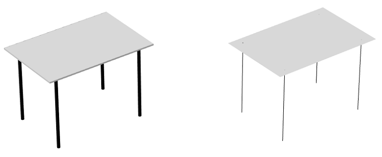
Left: Solid geometry of a reading table. Right: Geometry created with the Shell and Beam interfaces.
More examples where a combination of structural interfaces can be used are:
- Structures that are thin in large regions but more three-dimensional at certain locations. A mixture of solids and shells can then significantly reduce the model size.
- Plates or shells having beams as stiffeners.
- Truss elements acting as reinforcement bars in a concrete structure.
- A thin layer of one material on top of another material. In this case, an idealization with shells or membranes covering the boundary of a solid can be useful.
How can we couple these interfaces in a model? Well, the answer is that in COMSOL Multiphysics, there are a number of possible ways to do this. Which method we choose mainly depends on the type of problem at hand. Next, we’ll have a look at these methods, one by one, and discuss the types of problems they can be used with.
Methods for Coupling Structural Mechanics Interfaces
Built-In Coupling Features
Editor’s note: COMSOL Multiphysics® version 5.3 has introduced an easier way to implement the couplings described in this section of the blog post. For more details about this functionality, see the Release Highlights page for the Structural Mechanics Module.
In order to illustrate the built-in coupling features, let’s consider the Model Library example of a Pratt truss bridge (also available online in the Model Gallery), which is modeled using the Shell and Beam interfaces. The figure below shows the geometry of a Pratt truss bridge. Here, 3D edges, shown in black, are modeled using the Beam interface and 3D boundaries, shown in gray, are modeled using the Shell interface.
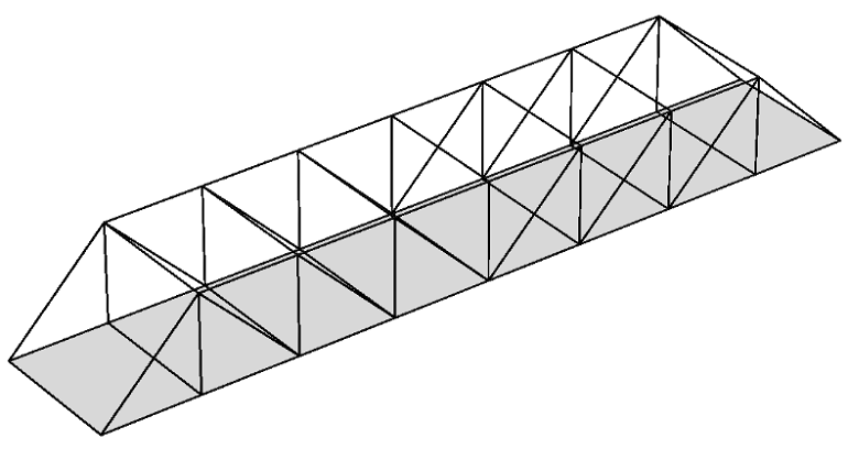
Geometry of a Pratt truss bridge, modeled using the Beam and Shell interfaces.
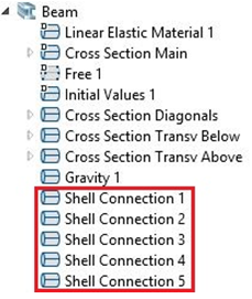
To couple the Shell and Beam interfaces in this model, we have utilized the built-in Beam-Shell coupling feature. Below, I have summarized the steps for using a Beam-Shell coupling:
- In the Beam interface, use the Shell Connection nodes for the edges that are common to the Shell and Beam interfaces.
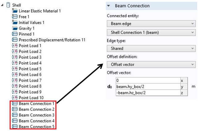
- In the Shell interface, use Beam Connection nodes on the common edges. You can also define an offset in the connection in the settings window. This is done to account for the fact that, in real life, the supporting beams are located below the concrete roadway.
The following built-in couplings are available and can be used in a similar manner as described above:
- Shell Edge to Solid Boundary (3D)
- Shell Boundary to Solid Boundary (3D)
- Beam Point to Solid Boundary (2D)
- Beam Edge to Solid Boundary (2D)
- Beam Edge to Shell Edge (3D)
- Beam Point to Shell Boundary (3D)
- Beam Point to Shell Edge (3D)
Using Prescribed Displacement
Another way of coupling different physics interfaces is through a Prescribed Displacement node, where the displacement is forced to be the same as the displacement in another physics interface. An example of this coupling is the Model Library example of a concrete beam with reinforcement bars (also in the Model Gallery).
The figure below shows the geometry of the model. Here, the concrete (3D Domain, gray colored) is modeled using the Solid Mechanics interface, while the reinforced bars (3D Edges, black colored) are modeled using the Truss interface.
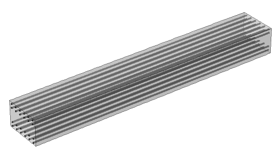
Geometry of a concrete beam that’s reinforced with steel bars. It was modeled using the Truss and Solid Mechanics interfaces.
In this model, individual rebars are modeled by adding a Truss interface to the Solid Mechanics interface, which was used for the concrete beam. The model uses a General Extrusion coupling operator, to make the displacement variables in the Solid Mechanics interface available for the Truss interface. The Prescribed Displacement node is then used in the Truss interface to provide the displacement variables from the Solid Mechanics interface, using the General Extrusion coupling operator that was defined earlier.
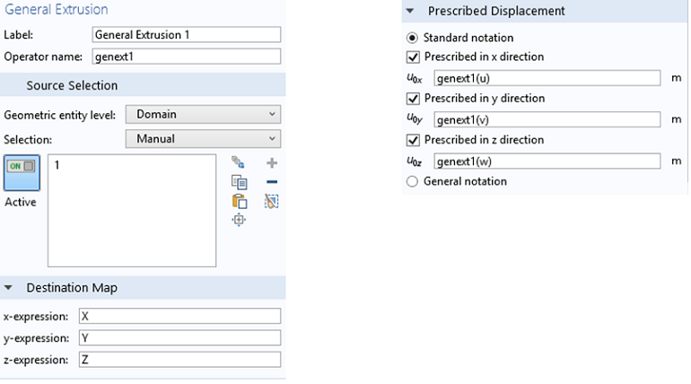
In this model, the mesh for the truss elements is not related to the mesh for the solid elements. The rebars just pass through the solid elements. This is why the coupling operator is needed.
Another modeling strategy would be to let the edges needed for the truss elements also be a part of the definition of the solid geometry.
Renaming Dependent Variables
Perhaps the easiest coupling method is to rename the displacement degrees of freedom so that these are the same for the interfaces that are to be coupled. This is sufficient, for example, when using membranes as cladding on a solid boundary or truss elements as reinforcement bars in a solid. Do note that this method works only when there is a union between the geometric entities of the structural interfaces being coupled.
Also notice the following exceptions:
- The shape functions used in the Beam interface have special properties. A beam cannot have the same degrees of freedom as another physics interface if the same edge or boundary is shared.
- The representation of rotations differs between the Shell and Plate interfaces and the Beam interface. Therefore, it is not possible to use common degree of freedom names for the rotational degrees of freedom.
Let’s apply this method to our model example of a concrete beam with reinforcement bars. We will modify the model to work with the same dependent variables for the Solid Mechanics and Truss interfaces. Follow the instructions below to solve the problem by renaming the dependent variables of the Truss interface.
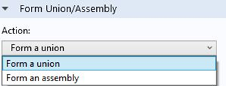
- In the current implementation of the model, there is an assembly of bars and a solid domain. We need to make a union of the edges and the solid domain in the geometry section.
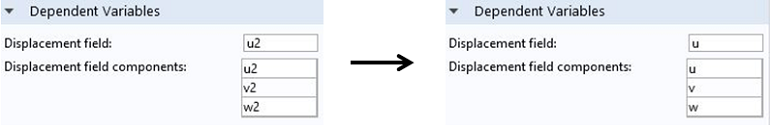
- Rename the dependent variables in the settings window of the Truss interface.
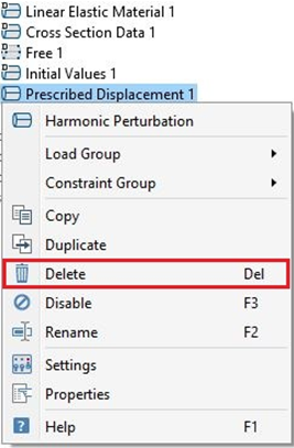
- Delete or disable the Prescribed Displacement 1 node in the Truss interface.
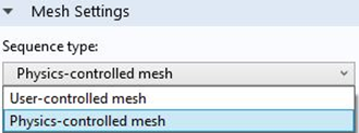
- Use a Physics controlled mesh.
We can now recompute the studies.
Multibody Attachments
An Attachment feature (requires the Multibody Dynamics Module) is available for the Multibody Dynamics, Solid Mechanics, Shell, and Beam interfaces. The attachment formulation is similar to the rigid connector, and all the selected boundaries or edges behave as if they were connected by a common rigid body. The various joints available with the Multibody Dynamics Module use these attachments to couple the interface with any other interface.
To clarify this method, let’s have a look at the Model Library model of vibrations in a washing machine assembly (also in the Model Gallery). In this model, a horizontal axis washing machine is modeled using the Multibody Dynamics and Shell interfaces. The outer housing of the assembly (gray colored) is made up of shell elements, while the inner components (differently colored) are rigid and are modeled using Rigid Domain nodes in the Multibody Dynamics interface.
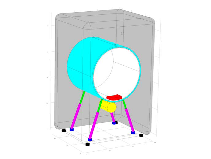
Geometry of a horizontal axis portable washing machine, which was modeled using the Multibody Dynamics and Shell interfaces (top, bottom, front, and left panels of the housing are hidden for better visualization).
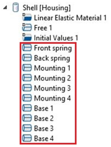
To couple the two interfaces, attachments are first created in the Shell interface. The instance below shows the attachment nodes created in the Shell interface.
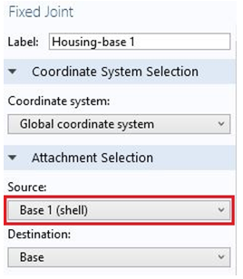
After defining the attachments in the Shell interface, fixed joints are created in the Multibody Dynamics interface. These fixed joints use the attachments from the Shell interface as the source and rigid bodies from the Multibody Dynamics interface as the destination, which results in a coupling of the two interfaces.
The screenshot below shows the settings window of one of the fixed joints with an attachment from the Shell interface as the source of the joint, and a Rigid Body node from the Multibody Dynamics interface as the destination of the joint.
A similar procedure is used to model the front and back springs present on the front and back panels of the housing. Have a look at the Model Gallery (or in the Model Library) entry called Vibration in a Washing Machine Assembly for more details about this model.
Editor’s note on 12/13/22: In version 6.1, the Rigid Domain feature has been renamed to Rigid Material.
Solver Settings When Coupling Structural Interfaces
Whenever there are multiple interfaces in a model, the default solver will generate a segregated solver sequence. However, it is not possible to solve a coupled model if the structural mechanics degrees of freedom are placed in separate segregated groups. The solution is to either replace the segregated solver with a fully coupled solver or place all structural mechanics degrees of freedom in one segregated step.
Further Reading
Apart from the models discussed above, the below models also demonstrate the coupling of structural interfaces:


Comments (3)
Yalcin Kaymak
February 20, 2015Thanks for very useful post.
Similar to structural mechanics, heat transfer module has also offer shell elements. Can I use the same method to combine shells and solids in heat transfer module?
Ignacio Garcia del Corral
August 1, 2015Thanks for the post!
Im trying to define a ball joint with two beam elements..but i dont know, how to define it.
could i get some help? thanks 🙂
Harsh Goel
October 27, 2020Hi
Is it possible to connect solid rotor and beam rotor interfaces? If yes pls pls pls pls tell how. Email: 26goelh@gmail.com