
Static mixers are well-established tools in a wide variety of engineering disciplines due to their efficiency, low cost, ease of installation, and minimal maintenance requirements. When evaluating whether a mixer can be used for a certain purpose, it is important to determine whether the resulting mixture is sufficiently uniform. In this blog post, we will discuss the setup of an app designed to quantitatively and qualitatively analyze the performance of a static mixer using the Particle Tracing Module.
The Foundations of the Laminar Static Particle Mixer Designer App
As a starting point for our Laminar Static Particle Mixer Designer app, we will consider the Particle Trajectories in a Laminar Static Mixer tutorial, which you can download from our Application Gallery. This model is designed to evaluate the mixing performance of a static mixer by computing particle trajectories throughout the device. To learn more about this tutorial and about mixer modeling in general, I encourage you to check out these previous blog posts:
- How to Simulate Particle Tracing in a Laminar Static Mixer
- Modeling of Laminar Flow Static Mixers
- Modeling Static Mixers
The geometry that is used in the tutorial referenced above is the same one that we will use within our app. Shown in the figure below, the model consists of a tube featuring three twisted blades with alternating rotations. The mixing blades are illustrated as gray surfaces, with the outline of the surrounding pipe also depicted. As particles are carried through the pipe by the fluid, they are mixed together by the static mixing blades.
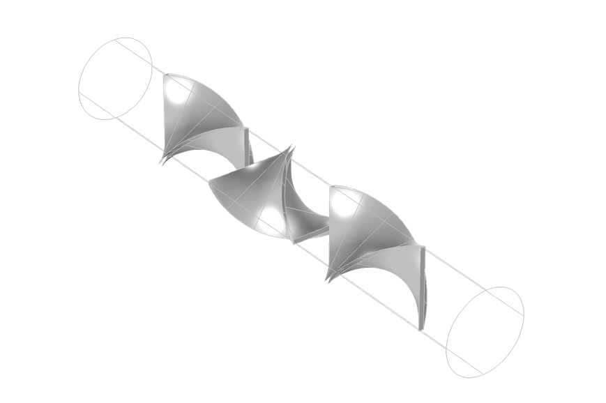
The geometry of the laminar static mixer model.
An App Designed to Study the Performance of a Static Mixer
Using our Laminar Static Particle Mixer Designer app, shown below, we can first compute the trajectories of particles as they move throughout the mixer. Then, using some built-in postprocessing tools, we can quantitatively and qualitatively evaluate how the mixer performs.

A screenshot of the user interface (UI) of the Laminar Static Particle Mixer Designer.
The app includes a large number of geometry parameters and material properties, with the option to create a mixer that utilizes one, two, or three helical mixing blades. Modifying the number of model particles and postprocessing parameters is also possible through the app’s advanced settings.
To better visualize the distribution of different species in the static mixer, we can release particles and compute their trajectories using the Particle Tracing for Fluid Flow interface. The particle positions are computed via a Newtonian formulation of the equations of motion, where the position vector components are calculated by solving a set of second-order equations:
(1)
where \mathbf{q} (SI unit: m) is the particle position, m_p (SI unit: kg) is the particle mass, and \mathbf{F}_t (SI unit: N) is the total force on the particles. The Newtonian formulation takes the inertia of the particles into account, allowing them to cross velocity streamlines.
In this model, the only force on the particles is the drag force, which is computed using the Stokes’ drag law:
(2)
\mathbf{F}_D &= \frac{1}{\tau_p} m_p \left(\mathbf{u}-\mathbf{v}\right)\\
\tau_p &= \frac{\rho_p d_p^2}{18 \mu}
\end{aligned}
where the following applies:
- \mathbf{v} (SI unit: m/s) is the particle velocity
- \mathbf{u} (SI unit: m/s) is the fluid velocity
- d_p (SI unit: m) is the particle diameter
- \rho_p (SI unit: kg/m^3) is the particle density
- \mu (SI unit: kg/(m\cdot s)) is the fluid dynamic viscosity
The Stokes’ drag law is applicable for particles with a relative Reynolds number much less than one; that is,
(3)
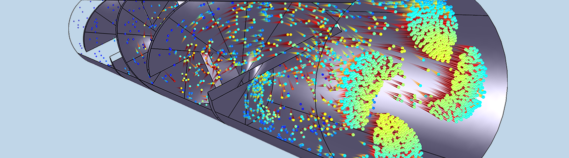
where \rho (SI unit: kg/m^3) is the density of the fluid. This is true in the present case. A representative sample of particles in the solution is depicted below. These particles are released at the bottom-right corner of the mixer and flow to the top-left corner. The color expression indicates the initial z-coordinate of the particles at the inlet, and it can be used to visualize the final positions of particles relative to their initial positions in the mixer cross section.
Plot illustrating particle trajectories in the static mixer.
Quantifying Static Mixer Performance with the Help of the Application Builder
To some extent, we can judge the uniformity of a mixture by observation alone. In this example, the mixing performance can be visualized by creating a phase portrait of the particle positions. In a phase portrait, particles can be plotted in an arbitrary 2D phase space — that is, they can be arranged in a 2D plot in which the axes can be user-defined expressions. Phase portraits are, for example, often used to plot particle position versus momentum in a certain direction, a phase space distribution.
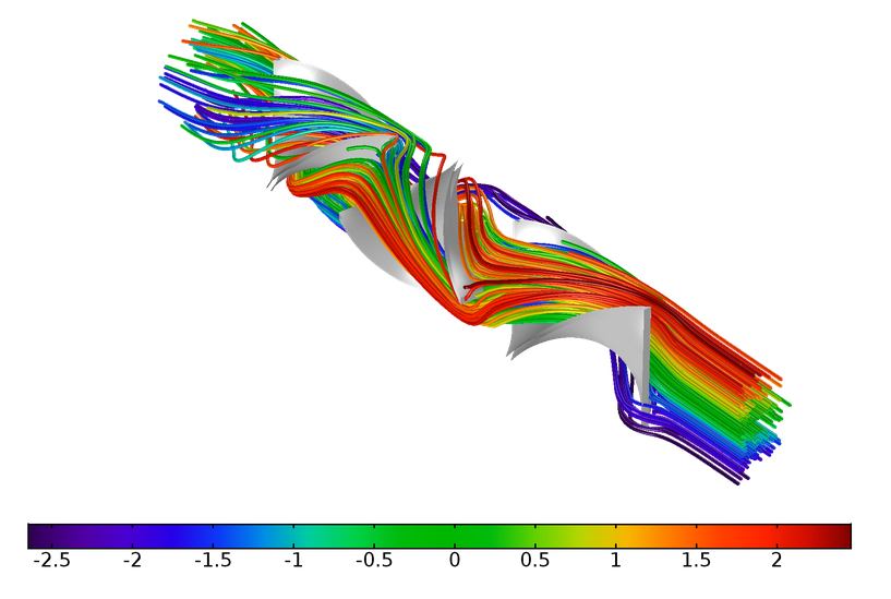
In the following animation, a phase portrait is used to observe the change in the transverse position of each particle as it moves throughout the mixer. Since the pipe is oriented in the y direction, the transverse directions are the x and z directions. The color expression denotes the quadrant that each particle occupied at the initial time; that is, dark blue particles were released with positive x– and z-coordinates, and so on.
A phase portrait indicates the transverse position of particles as they move throughout the mixer.
The phase portrait shows, qualitatively, that the particles are mixed together imperfectly at the outlet. There are still regions of higher or lower particle number density, along with clusters of particles of the same color — particles originating in the same quadrant — that can still be seen.
One potential drawback of the phase portrait is that it plots the particles in phase space at equal times, not at equal y-coordinates. This can produce a somewhat misleading visualization of the mixer, as some of the particles may move closer to the mixing blades and therefore potentially reach the outlet much later than other particles. An alternative option is to create a Poincaré map, which plots the intersection points of particles with a plane at a specified location.
In the following image, at each cut plane, the particles are colored according to whether they were released with positive (blue) or negative (red) initial x-coordinates. Once again, we can observe a clustering of red and blue particles at the outlet.
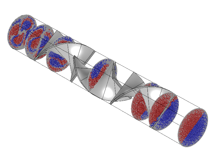
A Poincaré map shows the location of particles on a 2D plot.
Quite a lot of information about the mixer performance can be obtained from phase portraits and Poincaré maps, but most of it is too subjective for industrial applications. A human observer can judge approximately whether different species are completely unmixed, partially mixed, or well-mixed, but the lines between these definitions are hazy and difficult to quantify. For example, any observer can see that the previous images include pockets of particles of the same color, but it is much more difficult to assign a numerical value to describe how well-mixed they are.
Fortunately, the Application Builder and Method Editor provide the tools to create specialized, high-end postprocessing routines that can assign numeric values to the performance of a specific mixer geometry. A common metric for evaluating spatial uniformity of particles is the index of dispersion, defined as the ratio of the variance to the mean:
(4)
The mean and variance are computed by subdividing the outlet into a number of regions, or quadrats, of equal area. Because the outlet is circular, it can be subdivided into N_r annular regions of equal area by drawing concentric circles of radii
The annular regions can each be partitioned into N_{\phi} domains of equal area by drawing diameters at angles
The subdivision produces N_q=N_r N_{\phi} quadrats of equal area. Letting x_i denote the number of particles in the ith quadrat, the average number of particles in each quadrat is
The variance of the number of particles per quadrat is
The following method (p_computeIndexOfDispersion) is used in the app to compute the index of dispersion.
/*
 * p_computeIndexOfDispersion
 * This method computes the index of dispersion at the outlet.
 * The method is called in p_initApplication and in m_compute.
 */

// Get the x- and z-coordinates of the particles at the outlet
// and store them in matrices qx and qz, respectively.
model.result().numerical().create("par1", "Particle");
model.result().numerical("par1").set("solnum", new String[]{"14"});
model.result().numerical("par1").set("expr", "qx");
model.result().numerical("par1").set("unit", "m");
double[][] qx = model.result().numerical("par1").getReal();
model.result().numerical("par1").set("expr", "qz");
model.result().numerical("par1").set("unit", "m");
model.result().numerical("par1").set("solnum", new String[]{"14"});
double[][] qz = model.result().numerical("par1").getReal();

// Use the "at" operator to get the initial x-coordinates of all particles
// and store them in matrix qx0.
model.result().numerical("par1").set("expr", "at(0,qx)");
model.result().numerical("par1").set("unit", "m");
model.result().numerical("par1").set("solnum", new String[]{"14"});
double[][] qx0 = model.result().numerical("par1").getReal();

// The Particle Evaluation is no longer needed.
model.result().numerical().remove("par1");

double Ra = model.param().evaluate("Ra"); // Radius of the outlet
int Np = qx.length;                      // Number of particles
int Nr = nbrR;                            // Number of subdivisions in the radial direction
int Nphi = nbrPhi;                        // Number of subdivisions per quadrant in the azimuthal direction
int nbrQuad = Nr*4*Nphi;                  // Total number of quadrats (regions)
double deltaPhi = Math.PI/(2*Nphi);       // Angular width of each quadrat
int index = 0;
int ir = 0;
int iphi = 0;
int[] x = new int[nbrQuad]; // Array to store number of points per quadrat

// Begin loop over all particles
for (int i = 0; i < Np; ++i) {
  // Determine which quadrat each particle is in.
  ir = (int) Math.floor((Math.pow(qx[i][0], 2)+Math.pow(qz[i][0], 2))*Nr/Math.pow(Ra, 2));
  iphi = (int) Math.floor(Math.atan2(qz[i][0], qx[i][0])*Math.signum(qz[i][0])/deltaPhi);
  if (Math.signum(qz[i][0]) < 0) {
    iphi = (int) Math.floor((2*Math.PI-Math.atan2(qz[i][0], qx[i][0])*Math.signum(qz[i][0]))/deltaPhi);
  }
  index = 4*Nphi*ir+iphi;
  // Consider only half of the particles when evaluating mixer performance.
  if (qx0[i][0] < 0) {
    x[index] = x[index]+1;
  }
}
// compute the mean
double sum = 0;
for (int i = <0; i < nbrQuad; ++i) {
  sum += x[i];
}
// compute the variance
double xmean = sum/nbrQuad;
sum = 0;
for (int i = 0; i < nbrQuad; ++i) {
  sum += Math.pow(x[i]-xmean, 2);
}
indexOfDispersion = sum/xmean;
The last line of this method returns the index of dispersion. In general, a reduction of the index of dispersion corresponds to an improvement in the uniformity of the particle distribution. With the default parameters in the app, the index of dispersion is approximately 900 when three mixing blades are used, 1200 when two blades are used, and 1400 when only one blade is used. Thus, the index of dispersion quantitatively shows what we can see by looking at the plots: that a larger number of mixing blades produces a more uniform mixture of particles.
Simulation Apps Optimize the Analysis of Static Mixer Performance
Today, we have shown you how the Application Builder can advance your studies of static mixers. By creating an app, you can optimize the overall design workflow by spreading simulation capabilities to a wider audience, with the opportunity to gain a more accurate overview of mixing performance by assigning numerical values to different mixer geometries.
Interested in learning more about how to design simulation apps of your own? Be sure to check out the resources below.
Helpful Resources for Your App-Building Processes
- Try out the demo app presented here: Laminar Static Particle Mixer Designer
- For tips on how to enhance the structure and design of your simulation apps, as well as the user workflow, take a look at these blog posts:


Comments (0)