
In Part 3 of our series on multiscale modeling in high-frequency electromagnetics, let’s turn our attention to the receiving antenna. We’ve already covered theory and definitions in Part 1 and radiating antennas in Part 2. Today, we will couple a radiating antenna at one location with a receiving antenna 1000 λ away. For verification, we will calculate the received power via line-of-sight transmission and compare it with the Friis transmission line equation that we covered in Part 1.
Simulating the Background Field
In the simulation of our receiving antenna, we will use the Scattered Field formulation. This formulation is extremely useful when you have an object in the presence of a known field, such as in radar cross section (RCS) simulations. Since there are a number of scattered field simulations in the Application Gallery, and it has been discussed in a previous blog post, we will assume a familiarity with this technique and encourage you to review those resources if the Scattered Field formulation is new to you.
The Scattered Field formulation is useful for computing a radar cross section.
When comparing the implementation we will use here with the scattering examples in the Application Gallery, there are two differences that need to be referenced explicitly. The first is that, unlike the scattering examples, we will use a receiving antenna with a Lumped Port. With the Lumped Port excitation set to Off, it will receive power from the background field. This is automatically calculated in a predefined variable, and since the power is going into the lumped power, the value will be negative. The second difference, which we will spend more time discussing, is that the receiving antenna will be in a separate component than the emitting antenna and we will have to reference the results of one component in the other to link them.
Multiple Components in the Same Model
What does it mean when we have two or more components in a model? The defining feature of a component is that it has its own geometry and spatial dimension. If you would like to have a 2D axisymmetric geometry and a 3D geometry in the same simulation, then they would each require their own component. If you would like to do two 3D simulations in the same model, you only need one component, although in some situations it can be beneficial to separate them anyways.
Let’s say, for example, that you have two devices with relatively complicated geometries. If they are in the same component, then anytime you make a geometric change to one, they both need to be rebuilt (and remeshed). In separate components this would not be the case. Another common use of multiple components is submodeling, where the macroscopic structure is analyzed first and then a more detailed analysis is performed on a smaller region of the model. When we split into components, however, we then need to link the results between the simulations.
In our case, we have two antennas at a distance of 1000 λ. Separating them into distinct components is not strictly required, but we are going to do it anyways to keep things general. We will add in ray tracing later in this series and some users may find this multiple component method useful with an arbitrarily complex ray tracing geometry.
While we go through the details, it’s important that we have a clear image of the big picture. The main idea that we are pursuing in this post is that we first simulate an emitting antenna and calculate the radiated fields in a specific direction. Specifically, this is the direction of the receiving antenna. We then account for the distance between the antennas and use the calculated fields as the background field in a Scattered Field formulation for the receiving antenna. The emitting antenna is centered at the origin in component 1 and the receiving antenna is centered at the origin in component 2. Everything we will discuss here is simply the technical details of determining the emitted fields from the first simulation and using them as a background field in a second simulation.
Note: The overwhelming majority of the COMSOL Multiphysics® software models only have one component and only should have one component. Ensure that you have a sufficient need for multiple components in your model before implementing them, as there is a very real possibility of causing yourself extra work without benefit.
Connecting Components with Coupling Operators
There are a number of coupling operators, also known as component couplings, available in COMSOL Multiphysics. Generally speaking, these operators map the results from one spatial location to another. Said in another way, you can call for results in one location (the destination), but have the results evaluated at a separate location (the source). While this may seem trivial at first glance, it is an incredibly powerful and general technique. Let’s look at a few specific examples:
- We can evaluate the maximum or minimum value of a variable in a 3D domain, but call that result globally. This is a 3D to 0D mapping and allows us to create a temperature controller. Note that this can also be used with boundaries or edges, as well as averages or spatial integrations.
- We can extrude 2D simulation results to a 3D domain. This allows you to exploit translation symmetry in one physics (2D) and use the results in a more complex 3D model.
- We can project 3D data onto a 2D boundary (or 2D to 1D, etc.) A simple example of this is creating shadow puppets on a wall, but can also be useful for analyzing averages over a cross section.
As mentioned above, we want to simulate the emitting antenna (just like we did in Part 2 of the series) and calculate the radiated fields at a distance of 1000 λ. We then use a component coupling to map the fields to being centered about the origin in component 2.
Mapping the Radiated Fields
If we look at the far-field evaluation discussed in Part 2, we know that the x-component of the far field at a specific location is
The only complication is determining where to calculate the scattering amplitude. This is because component couplings need the source and destination to be locations that exist in the geometry. We don’t want to define a sphere in component 1 at the actual location of the receiving antenna, since that defeats the entire purpose of splitting the two antennas into two components. What we will do instead is create a variable for the magnitude of r, and then evaluate the scattering amplitude at a point in the geometry that shares the same angular coordinates, (\theta,\phi), as the point we are actually interested in. In the image below, we show the point where we would like to evaluate the scattering amplitude.
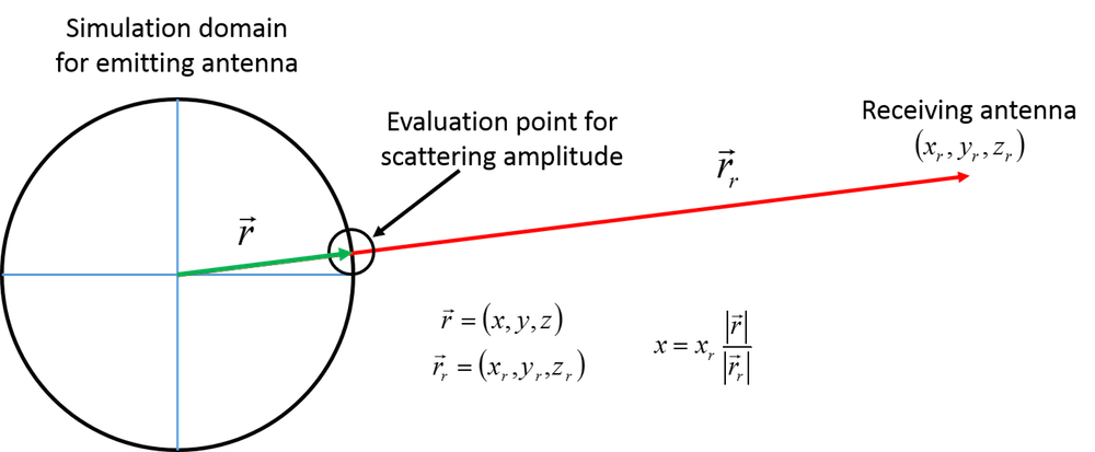
Image showing where the scattering amplitude should be calculated and how the coordinates of that point can be determined.
Defining the Point and Coupling Operator
We add a point to the geometry using the rescaling of the Cartesian coordinates shown in the above figure. Only x is shown in the figure, but the same scaling is also applied to y and z. For the COMSOL Multiphysics implementation, shown below, we have assumed that the receiving antenna is centered at a location of (1000 λ, 0, 0), and the two parameters used are ant_dist = |\vec{r}_1| and sim_r = |\vec{r}|.
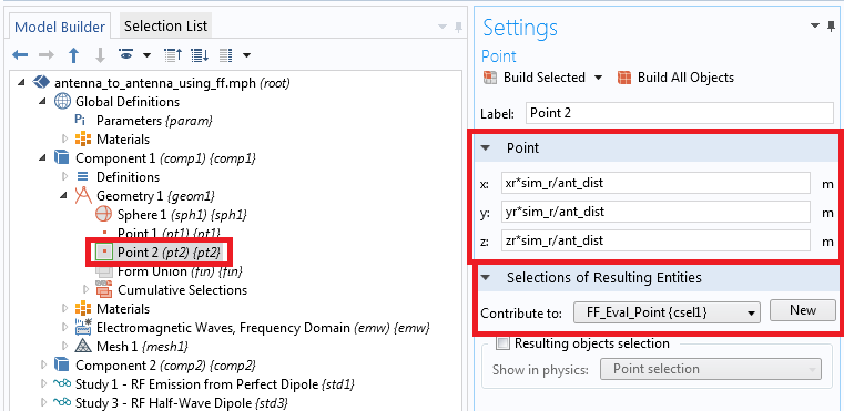
The required point for the correct scattering amplitude evaluation.
Note that we create a selection group from this point. This is so that it can be referenced without ambiguity. We then use this selection for an integration operator. Since we are integrating only over a single point, we simply return the value of the integrand at that point similar to using a Dirac delta function.
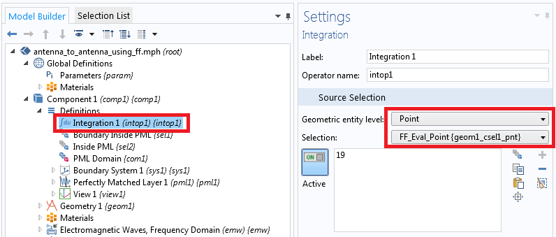
The integration operator is defined using the selection group for the evaluation point.
Running the Background Field Simulation in COMSOL Multiphysics®
The above discussion was all about how to evaluate the scattering amplitude at the correct location. The only remaining step is to use this in a background field simulation of the half-wavelength dipole discussed in Part 1. When we add in the known distance between the antennas, we get the following:
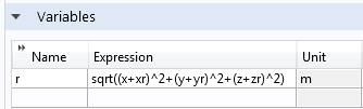
The variable definition for r. Note that this is defined in component 2.
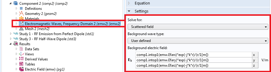
The background field settings.
In the settings, we see that the expression used for the background field in x is comp1.intop1(emw.Efarx)*exp(-j*k*r)/(r/1[m]), which matches the equation cited above. Also note that r is defined in component 2, while intop1() is defined in component 1. Since we are calling this from within component 2, we need to include the correct scope for the coupling operator, comp1.intop1(). The remainder of the receiving antenna simulation is functionally equivalent to other Scattered Field simulations in the Application Gallery, so we will not delve into the specifics here.
It is interesting to note that running either the emission or background field simulations by themselves is quite straightforward. All of the complication in this procedure is in correctly calculating the fields from component 1 and using them in component 2. All of this heavy lifting has paid off in that we can now fully simulate the received power in an antenna-to-antenna simulation, and the agreement between the simulated power and the Friis transmission equation is excellent. We can also obtain much more information from our simulation than we can purely from the Friis equation, since we have full knowledge of the electromagnetic fields at every point in space.
It is worth mentioning one final point before we conclude. We have only evaluated the far field at an individual point, so there is no angular dependence in the field at the receiving antenna. Because we are interested in antennas that are generally far apart, this is a valid approximation, although we will discuss a more general implementation in Part 4.
Concluding Thoughts on Coupling Radiating and Receiving Antennas
We have now reached a major benchmark in this blog series. After discussing terminology in Part 1 and emission in Part 2, we can now link a radiating antenna to a receiving antenna and verify our results against a known reference. The method we have implemented here can also be more useful than the Friis equation, as we have fully solved for the electromagnetic fields and any polarization mismatch is automatically accounted for.
There is one remaining issue, however, that we have not discussed. The method used here is only applicable to line-of-sight transmission through a homogeneous medium. If we had an inhomogeneous medium between the antennas or multipath transmission, that would not be appropriately accounted for either by this technique or the Friis equation. To solve that issue, we will need to use ray tracing to link the emitting and receiving antennas. In Part 4 of this blog series, we will show you how we can link a radiating source to a ray optics simulation.
Further Reading
- Browse previous posts in the Multiscale Modeling in High-Frequency Electromagnetics blog series


Comments (2)
Mona Nafari
October 22, 2017Thank you so much for such a useful explanations and models
Ashwinee Padvi
August 17, 2018When I change the source i.e. instead of Electric point dipole to dipole antenna, I get an error ‘Circular variable dependency detected, Variable: comp1.emw.nXEz’. What should be done for that?