
A paraboloidal solar dish can focus solar radiation onto a small target or cavity receiver. Because solar energy is collected over a large area, the incident heat flux at the receiver is extremely high. This thermal energy can then be converted to electrical energy or used to produce a chemical energy source, such as hydrogen. Today, we discuss strategies for computing the distribution of heat flux in the focal plane of a typical solar dish concentrator/receiver system.
Solar Thermal Energy: An Efficient Power Source
The basic operating principle of solar concentrator/receiver systems is that incoming solar radiation can be reflected by a curved surface, concentrated to a small area, and used to power a heat engine, such as a steam turbine. To focus solar radiation to the smallest area possible, the optimal shape of the reflector is a parabolic trough or a paraboloidal dish (shown below).
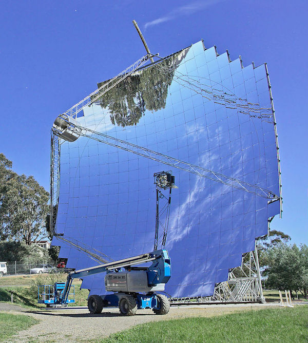
A paraboloidal dish for concentrated solar power and a maintenance crane. Image by Thennicke — Own work. Licensed under CC BY-SA 4.0, via Wikimedia Commons.
The maximum theoretical efficiency of a heat engine increases as the maximum temperature is increased, although beyond a certain temperature, the selection of materials may become too restricted for practical use. Therefore, great interest has been placed in predicting the operating temperature of the cavity receiver as accurately as possible.
An important figure of merit in predicting the temperature distribution is the concentration ratio (Ref. 1, Ref. 2), the ratio of incident flux on the surface of the cavity receiver to the ambient solar flux. The concentration ratio is increased when the radiation is focused to a smaller area or when losses in the system, such as absorption at the surface of the dish, are reduced. For some applications, such as hydrogen production, the uniformity of the heat flux has a large effect on the efficiency of the process. Therefore, we must consider how the concentration ratio varies over the surface of the receiver.
The receiver may have a variety of different shapes, several of which are investigated in Ref. 1, but for this post, we’ll assume that we’re just interested in the heat flux in the focal plane of the solar dish.
Predicting the Concentration Ratio of an Idealized Solar Collector
Ideally, a parabolic reflector can focus rays to a point. However, many perturbations prevent this idealized behavior from happening, even within the context of geometrical optics in which we neglect diffraction.
Let’s take a look at some of the perturbations in the system that can limit the focusing capability of a parabolic reflector.
Absorption
A fraction of the incident solar energy will be absorbed, not reflected, by the parabolic mirror. Even a new mirror absorbs some fraction of the incident energy, and years of wear and tear can further degrade its performance. The case described in Ref. 3 is a typical example.
Surface Roughness
A real mirror is not perfectly smooth. In a parabolic dish, there is always some deviation in the surface normal direction from the ideal case. This causes the solar radiation to be imperfectly focused, spreading the heat flux over a larger region in the focal plane.
Sunshape
If the Sun were an extremely small radiation source, then all of the incoming solar rays would be nearly parallel. However, this is not the case. Even at a distance of roughly 150 million kilometers, the Sun is still large enough that rays coming from different parts of the solar disk make significant angles with each other, so an angular spread in the Sun’s rays can still be observed. On Earth, the rays coming from the solar disk form a cone with a half-angle of about 4.65 mrad. Some additional radiation comes from the circumsolar region, the luminous region surrounding the Sun, but circumsolar radiation will not be considered in this example.
Taken broadly, the term sunshape refers to the effects of the finite size of the solar disk. In addition to causing a distribution of ray directions, another aspect of sunshape is the relative intensity of radiation from different parts of the solar disk (Ref. 4). Radiation from the center of the solar disk is usually brighter than radiation emitted from the outside of the disk, a phenomenon called solar limb darkening (Ref. 5). With the Ray Optics Module, the effect of the finite size of the Sun can be considered, either with or without accounting for the solar limb darkening effect.
Like surface roughness, the effects of sunshape tend to spread the incident heat flux over a larger region in the focal plane. The following plots show the concentration ratio in the focal plane for an ideal reflector (accounting for finite solar diameter only; see Ref. 2) and for a real reflector (accounting for finite solar diameter, solar limb darkening, surface roughness, and absorption, as in Ref. 1). The dish has a 45-degree rim angle and a focal length of 3 m.
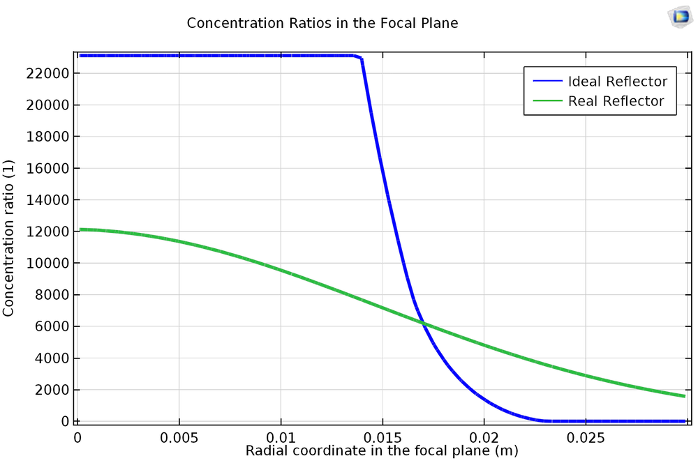
The concentration ratios in the focal plane for ideal and real reflectors.
A Monte Carlo Ray Tracing Solution
Several different computational models can be used to predict the concentration ratio in the focal plane of the dish. Monte Carlo ray tracing simulations have been used to account for finite source diameter, solar limb darkening, surface roughness, and absorption by the dish (Ref. 1). A semi-analytical model can also be used to compute a more idealistic solution, in which the finite size of the Sun is taken into account but solar limb darkening, surface roughness, and absorption are neglected (Ref. 2).
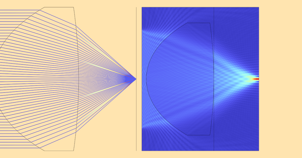
Using the Ray Optics Module, you can release the reflected solar radiation directly from the surface of the dish using the Illuminated Surface feature. After the rays reach the receiver, you can compute the heat flux in the focal plane using the Deposited Ray Power feature.
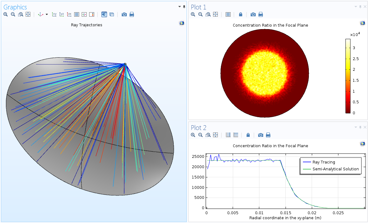
The trajectories of reflected rays (left), concentration ratio in the focal plane (top right), and azimuthally averaged concentration ratio as a function of radial position (bottom right).
Reporting the Concentration Ratio
As is usually the case with Monte Carlo simulations, the concentration ratio in the focal plane does include some numerical noise resulting from the random nature of the initial ray directions. Some of the built-in smoothing options can be used to improve the quality of the resulting plots. Increasing the number of rays in the simulation is another approach to smoothing out the statistical noise. Alternatively, a General Projection component coupling can be used to compute the average value of the concentration ratio as a function of radial position in the focal plane by integrating over all azimuthal angles:
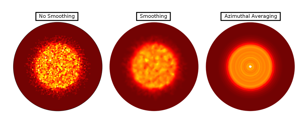
A comparison of the raw data (no smoothing), smoothed concentration ratio, and azimuthally averaged ratio.
The azimuthal averaging fails at the center (where integration takes place over an infinitesimally short distance), but at other locations, it gives a fairly accurate, uniform-looking representation of the concentration ratio in the focal plane.
The solutions for the ideal and real reflector are shown side-by-side below. The result for the ideal reflector is compared to a semi-analytical solution (Ref. 2), while the result for the real reflector is compared to published Monte Carlo ray tracing data from Ref. 1. The results are found to be in good agreement with the literature. The statistical noise could be further reduced by increasing the number of rays in the simulation.

Further Resources on Solar Concentrators and Ray Optics
- For a more detailed discussion of the solar limb darkening models and the semi-analytical solution used in Ref. 2, download the Solar Dish Receiver tutorial from the Application Gallery
- Read about the new features of the Ray Optics Module included with the latest version of COMSOL Multiphysics, version 5.2a
- Learn about other applications of ray optics simulation on the COMSOL Blog
References
- Y. Shuai, X-L. Xia, and H-P. Tan, “Radiation performance of dish solar concentrator/cavity receiver systems,” Solar Energy, vol. 82, pp. 13–21, 2008.
- S. M. Jeter, “The distribution of concentrated solar radiation in paraboloidal collectors,” Journal of Solar Energy Engineering, vol. 108, pp. 219-225, 1986.
- G. Johnston, “Focal region measurements of the 20 m2 tiled dish at the Australian national university,” Solar Energy, Vol. 63, No. 2, pp. 117-124, 1998.
- M. Schubnell, “Sunshape and its influence on the flux distribution in imaging solar concentrators,” Journal of Solar Energy Engineering, vol. 114, pp. 260-266, 1992.
- D. Hestroffer and C. Magnan, “Wavelength dependency of the Solar limb darkening,” Astron. Astrophysl, vol. 333, pp. 338-342, 1998.

Comments (11)
mona aghaee
January 29, 2018Hi,
I have problem modeling radiation heat transfer in a slab. A constant radiation hits an slab and part of that is transferred through the slab, part is absorbed within the slab and part is reflected. How should I model this? I already know the absorptance, reflectance and transmittance coefficients of the slab. Please advise.
Thanks
Mona
Abhinay Soanker
June 16, 2018Hi,
I have few questions regarding Ray tracing module in specific to solar dish tutorial:
1) I would like to know if this ray tracing simulation for solar dish is using Monte Carlo method to determine the Concentration ratio and flux distribution on the receiver?
2) Under Illuminated surface settings: “Number of rays per release” used in the module is equivalent to the Number of rays to be traced?
3) Under Ray properties settings: Since the source used is the sun and it has electromagnetic rays of different wavelength, why is “vacuum wavelength” of 660[nm] is used?
Christopher Boucher
June 29, 2018Hi Abhinay, thanks for reading!
1) Yes, I’d consider the approach in this tutorial to be a Monte Carlo method, since the perturbations from surface roughness and solar limb darkening phenomena are randomly sampled from probability distribution functions.
2) Usually it is true that the “Number of rays per release” is the total number of rays traced. If you have multiple ray sources then the total number is instead the sum of the “Number of rays per release” for each feature. Furthermore, some features allow you to specify both a number of release positions and a number or rays per release position, and then the total number of rays would be the product of these two values. These unique situations are discussed in the User’s Guide.
3) You do have a point here: the solar limb darkening model used in the second study has some wavelength dependence. In this case the wavelength distribution of the solar radiation didn’t significantly change the solution, so we allowed the light to be monochromatic so that we could better emphasize other parts of the model setup that had more noticeable effects on the concentration ration for the dish/receiver system.
Chris
Yassir Alamri
September 30, 2018Hi Chris,
Do we have in COMSOL results any parameter that can use to quantify the value of the radiation uniformity on the receiver?
This parameter will be used as a measure for the whole optical system performance, i.e. to provide us with a quantified measure of why this geometrical configuration is better than others, also it can allow us to optimize the system design and performance.
Kind regards
Inderjeet Singh
October 16, 2018Hi,
I have one question related to the design of the concentrator and receiver like; 1) can we increase the number of receiver and collector from one stage to two stage.
Inderjeet Singh
October 16, 2018One more question sir,
can we create roughness inside the receiver using COMSOL software?
Christopher Boucher
October 18, 2018Hi Yassir, thanks for reading. The plot of the “Concentration ratio” in this model is one way to measure the spatial uniformity on the receiver, just by observing how flat the “plateau” in this plot is. If instead you’d like a scalar figure-of-merit for the spatial uniformity, you could define one using a combination of Average and Integral component couplings defined over the receiver surface.
Christopher Boucher
October 18, 2018Hi Inderjeet, thanks for reading. With the Geometrical Optics interface, rays can be reflected any number of times. As for your second question, roughness inside the receiver could be modeled, by prescribing a combination of diffusive and specular reflection, or you could use the “General Reflection” boundary condition to implement a more sophisticated model of surface roughness.
Yassir Alamri
November 7, 2018Hi Christopher
Thanks for answering.
I would like to use the second option that you have suggested (scalar figure-of-merit for the spatial uniformity) by define one using a combination of Average and Integral component couplings defined over the receiver surface.
There is any tutorial in COMSOL showing how to use and implement these features to measure the uniformity?
Thanks again for your kind help.
Yassir
Kambiz Mozafarinia
April 7, 2019Hi
I have 2 questions. Please answer. 1_ How can I change the angle of light to the dish to 90 degrees? 2_How can I set the diameter of the dish apart from the focal length?
Thanks.
Edoardo Montà
December 11, 2019Hi Christopher,
I have a question regarding the solar dish model: is it possible to evaluate the temperature distribution in the focal plane?
I noticed that in the “Results” section, by adding “2D plot group”, a temperature map of the focal plane can obtained, but it is necessary to insert a specific formula in the form “gop.wall1.bsrc1……”.
Do you know the exact expression that should be written?
Thanks for your help,
Edoardo