

This post begins a comprehensive blog series where we will look at several approaches to multiscale modeling in high-frequency electromagnetics. Today, we will introduce the supporting theory and definitions that we will need. In subsequent posts, you will learn how to implement multiscale modeling of high-frequency electromagnetics for different scenarios in the COMSOL Multiphysics® software. Let’s get started…
Practical Scope: Antennas and Wireless Communication
Multiscale modeling is a challenging issue in modern simulation that occurs when there are vastly different scales in the same model. For example, your cellphone is approximately 15 cm, yet it receives GPS information from satellites 20,000 km away. Handling both of these lengths in the same simulation is not always straightforward. Similar issues show up in applications such as weather simulations, chemistry, and many other areas.
While multiscale modeling can be a general topic, we will focus our attention on the practical example of antennas and wireless communication. When we wirelessly transmit data via antennas, we can break the operation down into three main stages:
- An antenna converts a local signal into free space radiation.
- The radiation propagates away from the antenna over relatively long distances.
- The radiation is detected by another antenna and converted into a received signal.

Modern communications require long-distance wireless data transfer via antennas.
The two length scales that we will consider for this process are the wavelength of the radiation and the distance between the antennas. To use a specific example, FM radio has a wavelength of approximately three meters. When you listen to the radio in your car, you are often ten km or more away from the radio tower. Because many antennas, such as dipole antennas, are similar in size to a wavelength, we will not consider this to be another distinct length scale. As a result, we have one length scale for the emitting antenna, a different length scale for the signal propagation from source to destination, and then the original length scale again for the receiving antenna.
Let’s go over some of the most important equations, terms, and considerations when working with multiple scales in the same high-frequency electromagnetics model.
The Friis Transmission Equation
The Friis transmission equation calculates the received power for line-of-sight communication between two antennas separated by a lossless medium. The equation is
where the subscripts r and t discriminate between the transmission antenna and the receiving antenna, G is the antenna gain, P is the power, \Gamma is the reflection coefficient for impedance mismatch between antenna and transmission line, p is the polarization mismatch factor, λ is the wavelength, r is the distance between the antennas and is associated with the so-called free-space path loss, and \theta and \phi are the angular spherical coordinates for the two antennas.
Note that we have explicitly included two impedance mismatch terms, and so:
- Pt refers to the power provided to a transmission line attached to an emitting antenna
- Pr refers to the power received from a transmission line attached to a receiving antenna
The Friis transmission equation is derived in many texts, so we will not do so again here.
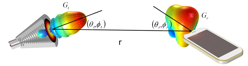
A visualization of the gain for a transmitting and receiving antenna. When using the Friis transmission equation, we require the orientation of each antenna for correct gain specification. The distance between the antennas is r.
Spherical Coordinates
Let’s now discuss spherical coordinates \left(r,\theta,\phi\right), since they are incredibly useful for antenna radiation and we will use them repeatedly. Starting from the Cartesian coordinates (x, y, z), we can easily express these as follows.
r& = sqrt(x^2 + y^2 + z^2)\\
\theta& = acos(z/r)\\
\phi& = atan2(y,x)
\end{align}
For convenience, we have used the actual COMSOL Multiphysics commands — sqrt(), acos(), and atan2(,) — instead of their mathematical symbols. In our simulation setup, we will also make use of the Cartesian components of the spherical unit vector \hat{\theta}.
\hat{\theta_x}& = cos(\theta)cos(\phi)\\
\hat{\theta_y}& = cos(\theta)sin(\phi)\\
\hat{\theta_z}& = -sin(\theta)
\end{align}
Similar assignments can be made for the Cartesian components of \hat{r} and \hat{\phi}, but \hat{\theta} is the most important for our purposes. This will be discussed later in this blog series when we cover ray optics.
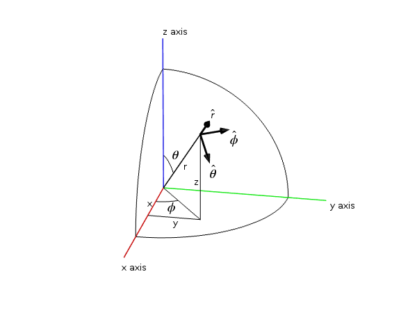
A given point shown in both Cartesian (x, y, z) and spherical \left(r,\theta,\phi\right) coordinates. The unit vectors for the spherical coordinates are also included. Note that the spherical unit vectors are functions of location.
The Poynting Vector and Radiation Intensity
We are generally interested in the radiated power from antennas. The power flux in W/m2 is represented by the complex Poynting vector \vec{S}=\frac{1}{2}\vec{E}\times\vec{H}^*.
Many antenna texts also use radiation intensity, which is defined as the power radiated per solid angle and measured in W/steradian. Mathematically speaking, this is U(\theta,\phi)=r^2\operatorname{Re}(\vec{S}\cdot\hat{r})=\frac{dP}{d\Omega}. For clarity, we have included two conventions here, as it is common to use U(\theta,\phi) in electrical engineering, while physicists will generally be more familiar with \frac{dP}{d\Omega}. We can then calculate the radiated power by integrating this quantity over all angles.
Gain and Directivity
Gain and directivity are similar in that they both quantify the radiated power in a given direction. The difference is that gain relates this radiated power to the input power, whereas directivity relates this to the overall radiated power. Put more simply, gain accounts for dielectric and conductive losses and directivity does not. Mathematically, this reads as G\left(\theta,\phi\right)=4\pi\frac{U\left(\theta,\phi\right)}{P_{in}} and D\left(\theta,\phi\right)=4\pi\frac{U\left(\theta,\phi\right)}{P_{rad}} for gain and directivity, respectively. Pin is the power accepted by the antenna and Prad is the total radiated power. While both quantities can be of interest, gain tends to be the more practical of these two as it accounts for material loss in the antenna. Because of its prevalence and usefulness, we also include the definition of gain (in a given direction) from “IEEE Standard Definitions of Terms for Antennas”, which is: “The ratio of the radiation intensity, in a given direction, to the radiation intensity that would be obtained if the power accepted by the antenna were radiated isotropically.”
IEEE also includes three notes about gain in their definition:
- “Gain does not include losses arising from impedance and polarization mismatches.”
- “The radiation intensity corresponding to the isotropically radiated power is equal to the power accepted by the antenna divided by 4π.”
- “If an antenna is without dissipative loss, then in any given direction, its gain is equal to its directivity.”
Gain, Realized Gain, and Impedance Mismatch
In practice, an actual antenna will be connected to a transmission line. Because the antenna and the transmission line may not have the same impedance, there can be a loss factor due to impedance mismatch. The realized gain is simply the gain when accounting for impedance mismatch. Mathematically, this is G_{realized} = \left(1-|\Gamma|^2\right)G, where \Gamma = \frac{Z_c-Z}{Z_c + Z} is the reflection coefficient from transmission line theory, Zc is the characteristic impedance of the transmission line, and Z is the impedance of the antenna.
When using a lumped port with a characteristic impedance in COMSOL Multiphysics, the far-field gain that is calculated corresponds to the IEEE realized gain. This is important to mention explicitly, since various definitions of gain have changed over the last few decades. Starting with COMSOL Multiphysics version 5.3, which will be released in 2017, the variable names in the COMSOL software will be changed to match the IEEE definitions.
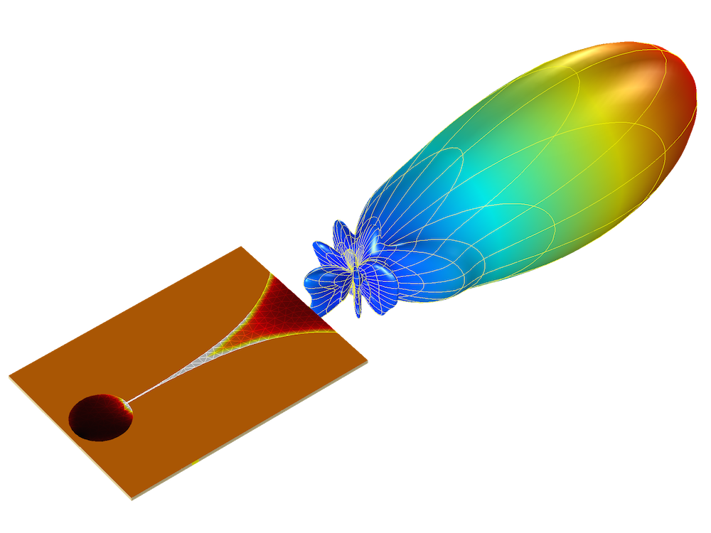
The realized gain and electric field from a Vivaldi antenna, simulated using COMSOL Multiphysics and the RF Module. You can find the Vivaldi Antenna tutorial model in the Application Gallery.
Receiving Antennas, Lorentz Reciprocity, and Received Power
The terms we have discussed so far have referred to antennas emitting radiation, but they are also generally applicable to receiving antennas. The reason we have put more emphasis on emission thus far is because antennas generally obey reciprocity (the Lorentz reciprocity theorem is a fixture in most antenna textbooks). Reciprocity means that an antenna’s gain in a specific direction is the same regardless of whether it is emitting in that direction or receiving a signal from that direction. Practically speaking, you can calculate the gain in any direction from a single simulation of an emitting antenna, which is easier than simulating the inverse process for each desired direction.
When we talk about receiving antennas, we are often interested in calculating the received power for an incoming signal. This can be done by multiplying the effective area, A_e=\frac{\lambda^2}{4\pi}G, of the antenna by the incident power flux and accounting for impedance mismatch in the line, yielding P_{rec} = \frac{\lambda^2}{4\pi}\left(1-|\Gamma|^2\right)G|\vec{S}|. As you may expect, this bears a striking similarity to several terms of the Friis transmission equation.
Emitter Example: A Perfect Electric Dipole
Today, we will talk about one type of emitter: the perfect electric point dipole. Depending on the literature, you may have seen this referred to as a perfect, ideal, or infinitesimal dipole. This emitter is a common representation of radiation for electrically small antennas. The solution for the field is
where \vec{p} is the dipole moment of the radiation source (not to be confused with the polarization mismatch) and k is the wave vector for the medium.
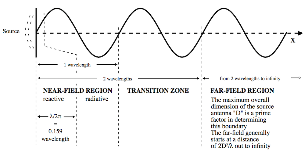
One breakdown of the various regions for the electromagnetic field generated from an electrically small antenna.
In this equation, there are three factors of 1/rn. The 1/r2 and 1/r3 terms will be more significant near the source, while the 1/r term will dominate at large distances. While the electromagnetic field will be continuous, it is common to refer to different regions of the field based on the distance from the source. One such distribution for an electrically small antenna is shown above, although there are other conventions that refer to the magnitude of kr.
Later, we will see how to calculate the fields at any distance from a given source, but the most important region for antenna communications is the far field or radiation zone, which is the region farthest away from the source. In this region, the fields take the form of spherical waves, \sim exp(-jkr)/r, a fact that we will take advantage of.
We will now split up the E-field equation above into two terms. For simplicity, we will call the 1/r term the far field (FF) and the 1/r2 and 1/r3 terms the near field (NF).
\overrightarrow{E}& = \overrightarrow{E}_{FF} + \overrightarrow{E}_{NF}\\
\overrightarrow{E}_{FF}& = \frac{1}{4\pi\epsilon_0}k^2(\hat{r}\times\vec{p})\times\hat{r}\frac{e^{-jkr}}{r}\\
\overrightarrow{E}_{NF}& = \frac{1}{4\pi\epsilon_0}[3\hat{r}(\hat{r}\cdot\vec{p})-\vec{p}](\frac{1}{r^3}+\frac{jk}{r^2})e^{-jkr}
\end{align}
As mentioned before, we can calculate the radiated power in watts by integrating U(\theta,\phi)=r^2\operatorname{Re}(\vec{S}\cdot\hat{r})=\frac{dP}{d\Omega} over all angles. Note that only the far-field term will contribute to this integral, which is a primary reason why the far field is of practical interest to antenna engineers. The total power radiated from a point dipole is P_{rad} = \frac{c^2Z_0k^4}{12\pi}|\vec{p}|^2, where Z0 is the impedance of free space and c is the speed of light. The maximum gain is 1.5 and is isotropic in the plane normal to the dipole moment (e.g., the xy-plane for a dipole in \hat{z}).
A note on units: The equations above are given with the traditional definition of the dipole moment \vec{p}=\int{\vec{r}\rho(\vec{r})d\vec{r}} in Coulomb*meters (Cm). In antenna and engineering texts, it is common to specify an infinitesimal current dipole in Ampere*meters (Am). COMSOL Multiphysics follows the engineering convention. The two definitions are related by a time derivative, so for a COMSOL software implementation, the dipole moment \vec{p} should be multiplied by a factor of j\omega to obtain the infinitesimal current dipole.
Receiver Example: A Half-Wavelength Dipole
We will use a perfectly conducting half-wavelength dipole as our receiving antenna.
A visual representation of radiation incident on a half-wavelength dipole antenna.
Many texts cover an infinitely thin wire, which has an impedance of \approx 73 \Omega and a directivity of D(\theta,\phi)\approx1.643\left[\frac{cos\left(\frac{\pi}{2}cos\theta\right)}{sin\theta}\right]^2. It is worth mentioning that the antenna impedance will change from these values for an antenna of finite radius. The receiving antenna we use here has a length of 0.47 λ and a length-to-diameter ratio of 100. With these values, we simulate an impedance of \approx 73 +3j \,\Omega, which is close to the infinitely thin value and also agrees reasonably well with experimental values. Regrettably, there is no theoretical value to compare to this number, but this highlights the need for numerical simulation in antenna design.
The comparison between the directivity of the infinitely thin dipole and our simulated dipole antenna is shown below. Because the antenna is lossless, this is equivalent to the antenna gain. You can download the dipole antenna model here.
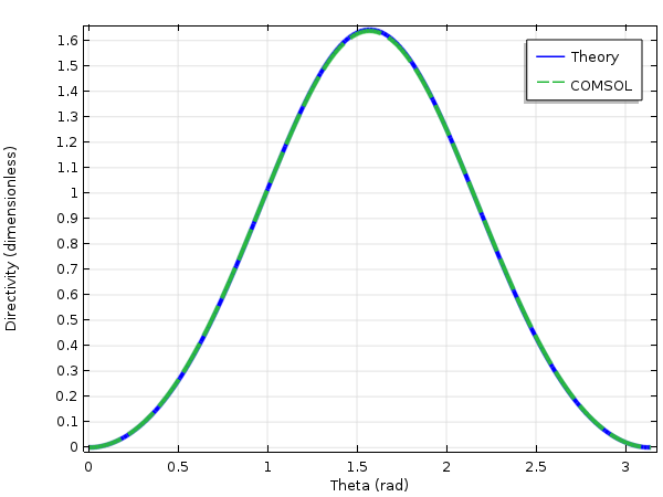
A comparison of the directivity for two half-wavelength antennas (oriented in z) as a function of theta. The COMSOL Multiphysics® simulation is of a finite radius cylinder and the theory is for an infinitely thin antenna.
Computing the Received Power
We can now use the Friis transmission equation to calculate the power that is emitted from a perfect point dipole and received by a half-wave dipole antenna. To use this equation, we simply need to know the gain and impedance mismatch (or realized gain), wavelength, distance between the antennas, and input power. Since we are using a point electric dipole, we have a dipole moment instead of input power and impedance mismatch. We can account for this by removing the impedance mismatch term and replacing the input power by the radiated power of the perfect electric dipole from above — effectively saying that power in equals power out.
If we assume that our emitter and detector are both located in the xy-plane, are polarization matched, and are separated by 1000 λ, as well as that the dipole moment of the emitter is 1 Am in \hat{z}, the Friis equation yields a received power of 380 μW. We will simulate this value in part 3 of this series for verification of our simulation technique. We can then use our simulation to confidently extract results and introduce complexity that the Friis equation cannot account for.
Concluding Thoughts
In this blog post, we have introduced the idea of multiscale modeling and discussed all of the relevant terms, definitions, and theory that we will need moving forward. For those of you with a strong background in electromagnetics and antenna design, this has likely been a quick review. If the concepts presented here are new to you, we strongly recommend further reading in a book on classical electromagnetics or antenna theory.
In the following blog posts, we will focus primarily on practical implementation of multiscale modeling in COMSOL Multiphysics and we will repeatedly refer to concepts discussed today.
Coming Up Next…
Stay tuned for more installments in our multiscale modeling blog series:
- In part 2, we will simulate the emission from a point electric dipole using the Electromagnetic Waves, Frequency Domain interface. We will discuss the Far-Field Domain node, which calculates the far-field radiation from a source, and show how the Electromagnetic Waves, Frequency Domain interface can be coupled to the Electromagnetic Waves, Beam Envelopes interface to simulate fields in the intermediate zone.
- In part 3, we will simulate a point dipole radiating to a half-wavelength dipole antenna an arbitrary distance away. For verification, we will calculate the power received by the half-wavelength dipole antenna and verify our results using the Friis transmission equation.
- In part 4, we will couple our emitting source, the point electric dipole, to a ray optics simulation using the Geometrical Optics interface.
- In part 5, we will couple the two antennas using the Geometrical Optics interface. We will again verify our results and discuss how this more general method can account for inhomogeneous media and multipath transmission.


Comments (1)
Nirmal Paudel
January 12, 2017Awesome blog post Drew.