

Imagine bending a metallic paper clip back and forth until, after a few repetitions, it breaks entirely. This is one example of fatigue failure, the most common type of structural collapse. In more severe cases, such failure can lead to collapse or malfunction in structures like car exhaust pipes and aircraft jet engines. To better understand and predict fatigue failure in elastoplastic materials, we can use the COMSOL Multiphysics® software to accurately model both the materials and the fatigue process.
What Are Elastoplastic Materials?
Elastoplastic materials combine two principal types of behavior: elastic deformation, which is reversible deformation, and plastic deformation (or plasticity), which is irreversible and leaves a permanent deformation upon unloading. In order to model this type of material behavior, we need to use a constitutive relation that connects the stress state not only to the current strain state, but also to the previously accumulated plastic strains and to their development.
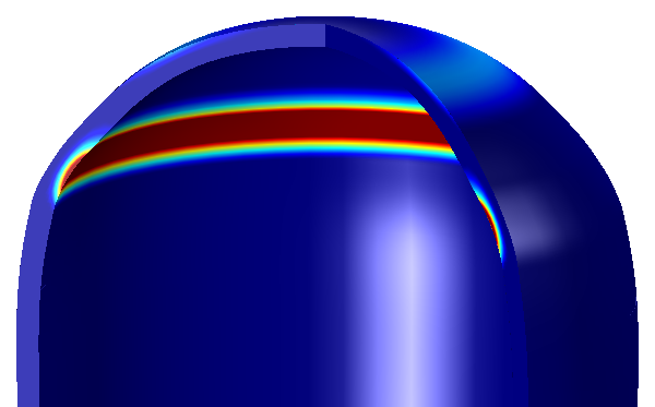
Plastic deformation in a pressure vessel subjected to internal pressure, showing the elastic region (dark blue) and some plasticity (red).
Generally, when there is an increase in stress and the initial yield stress (the elastic limit) is surpassed, the elastoplastic material is strained much more than for a corresponding stress increase in the elastic region. The material is hardened by plastic deformation, but the response in the plastic regime varies greatly among different materials.
For metallic materials, hardening is commonly described by three different types of behavior:
- Isotropic hardening, in which the yield surface expands with increasing stress. Loading in tension also hardens the material in compression
- Kinematic hardening, in which the yield surface translates, but stays the same size. Loading in tension will make the material softer in compression
- Mixed hardening, in which the yield surface both expands and translates
In the figures below, we can visualize the stress-strain relation for a uniaxial loading for the three types of hardening. In the first step, the material is stretched until a significant plastic strain is reached. At this point, the current yield stress, \sigma_{\textrm{y}}, is above the initial yield stress, \sigma_{\textrm{y0}}. So far, the stress-strain curve follows the same path for all three types of hardening. In the second step, the loading direction is reversed and the material is compressed until the onset of yielding in compression.
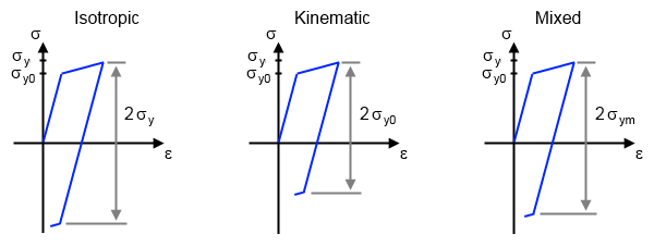
The stress-strain relation in a uniaxial load case for three hardening models: isotropic, kinematic, and mixed.
With isotropic hardening, a material can be compressed at most 2\sigma_{\textrm{y}} before the onset of reversed yielding. With kinematic hardening, a material can be compressed at most 2\sigma_{\textrm{y0}}. With mixed hardening, the compression is in between the two, having 2\sigma_{\textrm{y0}} < 2\sigma_{\textrm{ym}} < 2\sigma_{\textrm{y}}. Both kinematic and mixed hardening result in a so-called back stress or shift stress, which is a new stress level that is equally far from yielding in tension and compression. Before the onset of plasticity and in the case of isotropic hardening, the back stress is zero.
Besides this type of deformation hardening, some metallic materials also demonstrate more complex types of behavior. One example is viscoplasticity, where the plastic behavior is strain rate dependent.
Modeling Fatigue Failure in COMSOL Multiphysics®
You can access a collection of material models that can be used for modeling elastoplastic materials in the Nonlinear Structural Materials Module. Selecting a fatigue model, however, does not only depend on the material model, but also on the loading characteristics. We talk about the influence of loading conditions on the choice of fatigue model in a previous blog post.
When working with nonlinear materials such as elastoplastic materials, the material response of the first load cycle generally differs from the material response of the second cycle. This is caused by the first load cycle, which can both shift the yield surface and change the yield stress. The consecutive load cycles can then either oscillate around a new stress-strain state or cause further accumulation of inelastic strains. When studying fatigue, we must first find a stable load cycle, which is representative for the subsequent cycles. Therefore, when modeling elastoplastic materials, we often need to simulate several load cycles before reaching a stable load cycle.
We discuss the different types of load cycles in another blog post: Modeling Thermal Fatigue in Nonlinear Materials.
Let’s go over how to model fatigue in elastoplastic materials with two of the types of hardening, kinematic and isotropic hardening, using COMSOL Multiphysics.
Modeling Fatigue in Materials with Kinematic Hardening
Let’s take a look at the Elastoplastic Low-Cycle Fatigue of Cylinder with a Hole tutorial model. Here, the component is loaded beyond the point of yielding. The material experiences immediate stability, since a stable load cycle is obtained already during the second cycle. However, the stable load cycle consists of both elastic and plastic deformations. This is possible since the material is modeled with kinematic hardening. This means that the yield surface moves between two positions: tension and compression.
For most applications that involve kinematic hardening, a full elastoplastic analysis must be performed. The model size can be somewhat reduced by dividing the model into domains where plasticity develops and domains where only elastic deformation takes place. This method is useful because plasticity is computationally expensive to model, requiring us to evaluate an additional seven degrees of freedom as opposed to the three displacements in elastic materials.
It is common that fatigue failure originates from the presence of a notch. In this case, an approximate solution can be used; for example, the Neuber correction for plasticity based on the Ramberg-Osgood material model. Based on the elastic solution, this approximate method computes an elastoplastic stress-strain state at a notch. This method is fast, but the further away we move from the notch, the lower the accuracy of the results. This method is demonstrated in a related example model: Notch Approximation to Low-Cycle Fatigue Analysis of Cylinder with a Hole.
We can compare the two methods in the figures below. Due to high strain and multiaxial load conditions at the hole, we predict fatigue using the low-cycle-fatigue Smith-Watson-Topper (SWT) model. The results at the critical spot are similar for both methods. The computation time, on the other hand, differs significantly. For the elastoplastic model, computation time is a few minutes, compared to a few seconds for the notch approximation.
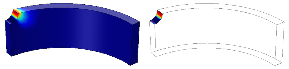
A low-cycle fatigue prediction, based on a full elastoplastic analysis (left) and a notch approximation (right). Results display the logarithm of the number of cycles to failure. The same color scale is used in both figures.
Modeling Fatigue in Materials with Isotropic Hardening
In another tutorial model, Standing Contact Fatigue, a surface-hardened material is subjected to a compressive load cycle. Affected by the hardening process, the tested material has three distinct layers with different material properties. The material is strong closest to the surface (the case), while it is weak deep inside (the core). In between, there is a thin transition layer where both the material properties and residual stress sharply change.
The plastic properties of the material differ through the depth. In the case layer, the hardening follows a linear isotropic model, while in the core, it follows an exponential hardening model. In the transition layer, the hardening function is exponential and parameterized. The function for the material parameters is chosen such that the material model of the transition layer at the interface with the case corresponds to the case model, and the interface with the core corresponds to the core model.
During the first load cycle, the material is compressed past the point of yielding and plasticity grows on the subsurface level. Since the yield surface expands in isotropic hardening, each consecutive load cycle that is not as high in magnitude as the first cycle will not introduce any further plasticity, thus the stable load cycle is elastic. Although high strains develop during the first load cycle, any consecutive cycle will result in small strain changes. It is therefore reasonable to assume that a stress-driven, high-cycle fatigue model is suitable for fatigue evaluation.
In the case of a predominantly compressive load, the Dang Van model is useful for fatigue modeling, since it takes the compressive mean stress into account. You can access the Dang Van model for these types of simulations in the Fatigue Module.
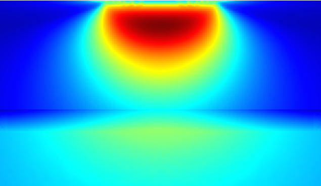
Fatigue prediction in a surface-hardened material. Fatigue usage factor is displayed. The highest risk of fatigue is in the near-surface case layer, with a lower risk of fatigue in the deep core layer.
By simulating fatigue in common types of elastoplastic materials with COMSOL Multiphysics, we can better understand and predict the occurrence of fatigue failure.
Additional Resources for Modeling Fatigue and Nonlinear Structural Materials
- Try it yourself: Download the tutorial models discussed in this blog post
- Learn more about applications for modeling nonlinear structural materials and fatigue on the COMSOL Blog


Comments (0)