
After recently encountering the equations of motion for rotating bodies for the first time, one of my sons came home with a number of interesting questions. His questions brought about a flashback, as I remembered sharing this sense of confusion when studying mechanics many years ago. In today’s blog post, I will present two COMSOL Multiphysics models — one of a gyroscope and one of a spinning top — that illustrate the remarkable properties of rotating bodies.
What Is a Gyroscope?
The gyroscope — a term coined by Léon Foucault during the middle of the 19th century — has been recognized as an instrument in science and engineering for nearly two hundred years. Its predecessor, the spinning top, has been known since ancient times, with uses as a toy, for gambling, and as an object with magic properties.
As an instrument, the gyroscope is valued for its precision in measuring and maintaining orientation. Such properties have facilitated its use in airplanes, spacecraft, and submarines, as well as within the sensors of inertial guidance systems.
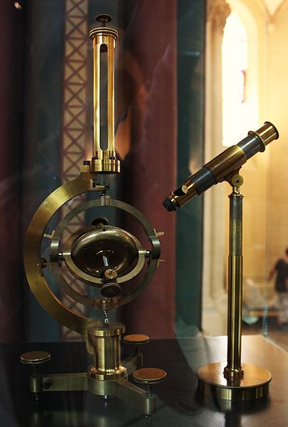
A replica of the first gyroscope.
The classical gyroscope is based on the law of conservation of angular momentum. A spinning body wants to maintain the orientation of its axis in the absence of external moments. The resistance to changing orientation when perturbed depends on the angular momentum, that is, the product of the angular velocity and the mass moment of inertia. When a moment that is not parallel to the axis of rotation is applied to the rotor, the effect can be quite surprising.
Note: Several types of devices exist today with the same purpose as the classical gyroscope, but they are based on different physical properties. Recent developments in physics and microscale engineering have made this possible.
As the schematic below illustrates, a gyroscope consists of a disc that is forced to spin with a high angular velocity around an axis. The axis is journaled in an inner ring called a gimbal. The inner gimbal is attached to the outer gimbal with another pair of journals. These journals have an axis that is positioned at a right angle to the spinning shaft. A third pair of journals attaches the outer gimbal to the frame. As a result, the rotor has three rotational degrees of freedom, one about each axis. Note that the frame is attached to the surroundings (i.e., the vessel).
If the frame is rotated around an arbitrary axis, the rotor axis strives to maintain its direction. While doing so, both gimbals are forced to rotate.
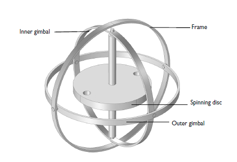
A sketch of a classical gyroscope.
Modeling Gyroscopic Effects in COMSOL Multiphysics
Using the Multibody Dynamics Module in COMSOL Multiphysics, we can simulate the mechanical properties of a gyroscope. Our Modeling Gyroscopic Effect tutorial model focuses on such studies. The example, which we will discuss next, is actually comprised of two models: a gyroscope and a spinning top.
The Gyroscope Model
Let’s begin with our gyroscope model. The geometry for the model includes four rigid bodies: the rotor, the two gimbals, and the frame. Steel is used as the material in the rotor, while aluminum is used in other parts. Because of these material choices, the rotor’s moment of inertia is large as compared to the supporting structure. The frame is given a prescribed rotation around an axis oriented at 90° from the rotor axis and at 45° from both gimbal journal axes. The frame rotation is harmonic with a magnitude of 2 rad and a frequency of 2 Hz. Each of the journals is modeled as a hinge joint.
Two different situations are addressed in the analysis to illustrate the effect of a rotor spinning on its orientation. In the first case, the rotor is not spinning. In the second case, an angular speed of 350 rad/s (3342 RPM) is prescribed as the initial value for the rotor.
The first animation below shows how the rotor is forced to change its orientation when it is not spinning. There is no gravity in the problem, and kinematically, it is possible for the rotor to maintain its orientation, so the rigid body dynamics of the system cause the change in the orientation of the rotor. In the second animation, we can see that the rotor essentially maintains its orientation since it is spinning.
Orientation of the rotor under the imposed rotation of the frame when the rotor is not spinning.
Orientation of the rotor under the imposed rotation of the frame when the rotor is spinning.
Plotted in the graph below is the inclination angle of the rotor axis, with the difference in stability shown. An angle error of about 1°, which occurs in the rotating case, may still not be useful in a precision instrument. Design changes, however, can reduce such deviation. In our example, the frame’s rate of rotation is rather high. The frame rotates approximately 115° and then back in the 0.25 seconds that are covered by the simulation study. To improve the stability of the axis orientation under such an external disturbance, a higher rotor speed or a heavier rotor is necessary.

Comparing the rotor axis inclination with and without spinning.
The Spinning Top Model
Shifting focus, let’s now look at the spinning top model. Here, we use only a single rigid body: the rotor from the previous example. The rotor axis is initially oriented at 20° from the vertical axis, and a gravity load is added. Further, an initial angular velocity is given to the rotor about its own axis. Together with the reaction force at the bottom, the gravity load creates a moment pointing out of the plane that is spanned by the rotor axis and the vertical axis.
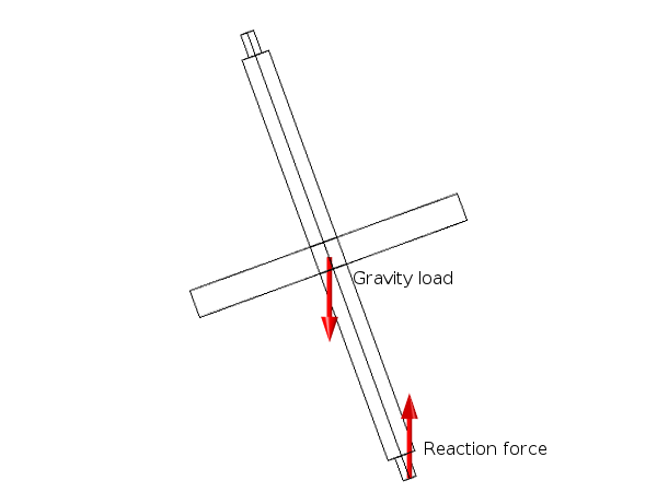
The force couple acting on the spinning top.
This moment causes an angular acceleration in the direction out of the plane, and the spinning top starts to alter its orientation. This change in orientation of the spinning top, together with the spinning about its own axis, causes a gyroscopic torque on the spinning top. Under the effect of gyroscopic torque, the tip of the spinning top slowly moves along a circular path. Such rotation of the rotor axis orientation is referred to as precession. The plot below illustrates the trajectory of the tip of the axis.
Trajectory of the tip of the axis for the spinning top.
As we can see, the wide circular path is overlaid by a smaller periodic disturbance — a movement known as nutation. The nutation depends on the initial conditions. Since the spinning top study begins with only a rotation around the rotor axis and no precession velocity, the initial conditions are not compatible with a pure precession movement. In a real physical system, damping would decrease the nutation amplitude over time.
Concluding Thoughts
When you want to solve problems of this type, it is important to limit the time step used in the analysis. Typically, the time step must be limited to correspond with a rotation angle of the order of a few degrees per time step. In the above examples, a time step of 0.1 ms is used. This corresponds to approximately 2° of rotation of the rotor around its axis during each time step.
You can download the tutorial model presented here from our Application Gallery. If you are interested in learning about another technology for designing MEMS gyroscopes, we encourage you to check out our Piezoelectric Rate Gyroscope tutorial model as well.


Comments (0)