

Optical devices such as monochromators and spectrometers can be used to separate polychromatic, or multicolored, light into separate colors. These devices have many applications in diverse areas that range from chemistry to astronomy. Using built-in tools in the Ray Optics Module, it is possible to model the separation of electromagnetic rays at different frequencies with a monochromator or spectrometer as well as analyze the resolution of such devices.
Editor’s note: This blog post was updated on January 20, 2023, to reflect new features and functionality in the COMSOL Multiphysics® software.
The Setup of a Basic Spectrometer
A spectrometer is a device that measures some property of radiation (e.g., its intensity or state of polarization) as a function of its frequency. Spectrometers can be designed for detecting radiation at a number of different frequency ranges. This extends from visible light to gamma rays and infrared radiation.
A basic spectrometer includes a lens or mirror to convert incoming light into a parallel (or collimated) beam along with a mechanism for separating the light into different frequencies. The device also features another lens or mirror to focus light of different frequencies at specific locations. If a narrow exit slit is used to only transmit radiation of a specific frequency, the device is referred to as a monochromator.
Spectrometers are widely used to analyze the composition of mixtures of chemicals. Each element releases photons in specific frequency ranges (collectively known as the element’s emission spectrum) as excited electrons return to lower energy states. Using known emission spectra, it is possible to determine the composition of a sample based on the radiation that it emits. Similarly, it is possible to analyze the composition of stars based on the radiation they emit and even estimate the redshift of very distant objects.
There are several ways to separate polychromatic light into individual colors. Early spectrometers often used a prism made of a material with a frequency-dependent refractive index n. Such materials are also called dispersive media. As light enters and leaves the prism, its direction of propagation is determined by Snell’s Law,
(1)
where the subscripts i and t denote the incident and refracted light, respectively. If the refractive index is frequency-dependent and the angle of incidence is nonzero, then the angle of refraction is also frequency-dependent. As a result, a collimated beam of polychromatic light will be separated, as illustrated below.
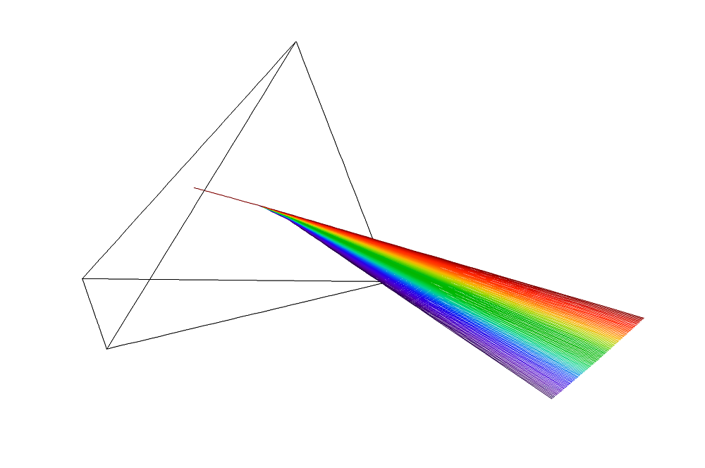
Diffraction of polychromatic light in the prism made of dispersive material.
Modern spectrometers typically use a diffraction grating instead of a prism containing a dispersive medium. A diffraction grating is a periodic arrangement containing a large number of identical unit cells. When an electromagnetic wave reaches the grating, it can only be transmitted and reflected in specific directions. These directions depend on the wavelength of the incident light and the width of a single unit cell d.
In order for reflected or refracted light to propagate in a certain direction, the waves from adjacent unit cells must interfere constructively with each other. For a reflected ray of free-space wavelength \lambda_0 with integer-valued diffraction order m, the angle of incidence \theta_i and angle of reflection \theta_r are related by
(2)
The reflection of rays from adjacent unit cells is illustrated below.
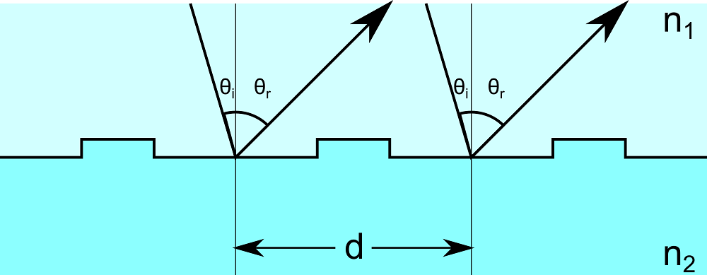
Light reflection from typical diffraction grating.
From Eq. (2), it is clear that if the diffraction order is nonzero, the direction of reflected radiation will depend on the free-space wavelength. This is the basic property of the grating that can be used to separate different frequencies of radiation.
Modeling the Czerny–Turner Configuration
We now use the COMSOL Multiphysics® software with the Ray Optics Module to model light propagation in a basic optical device. This example consists of two mirrors and a diffraction grating arranged in a crossed Czerny–Turner configuration.
Principle of Operation and Ray Trajectories
Incoming rays are released from a slit (1) with a conical distribution. The rays are reflected by a collimating mirror (2) so that all of the rays are parallel as they hit the diffraction grating (3). The reflected rays of diffraction order 0 travel along parallel paths because their angle of reflection is not wavelength-dependent. Because the different colors have not been separated, these rays are aimed away from the mirrors and ignored (4).
However, the rays of diffraction order 1 are reflected in different directions based on free-space wavelength. They are reflected by a focusing mirror (5) so that rays of different frequencies are focused at different points on a detector (6). If a narrow exit slit were placed at the detector, the resulting device would be a Czerny–Turner monochromator capable of transmitting radiation only in an extremely narrow frequency band.
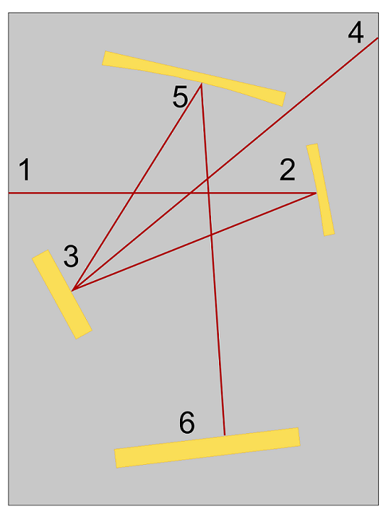

Schematic of an Czerny–Turner monochromator with annotations (left) and the calculated ray trajectories (right). The rays are colored according to their vacuum wavelength.
Modeling Tips and Best Practices
The key component of such a design is diffraction grating. To perform a ray optics calculation of the design, there is no need to create the grating’s complex microscale geometry. We can use a planar boundary with the Grating boundary condition and define its main parameters, such as the grating type (reflective in our case), grating orientation, and grating constant. Then we should add all desired diffraction orders (0 and 1 in our case) for a direct calculation via the Diffraction order subnodes.
Note that the reflected rays of diffraction order 0 won’t interact with any optical component, as they escape the system through the upper-right corner. These rays are thus no longer relevant to the solution and can be removed via the Ray Termination feature. This will simplify the model setup and postprocessing.

The Settings window for the Grating feature. You can also see the model geometry in the Graphics window.
Note that starting from COMSOL® version 5.2a there is no need to add an air or vacuum domain to encompass the rays; they can propagate in the void region outside of the geometry. Because of this, we can use a more minimalist geometry. Moreover, only the boundaries of the components should be meshed. In order to compute the ray paths as accurately as possible, we can resolve the mesh on the curved boundaries of the collimating mirror and the focusing mirror. On planar boundaries, a coarse mesh is acceptable. One way to quickly set up the mesh is to specify a very low curvature factor, which causes the mesh to be automatically refined near curved boundaries.
Spectral Resolution of the Device
Although the crossed Czerny–Turner configuration appears to focus rays of each frequency to a distinct point, rays of a single frequency are actually distributed over an area of small but nonzero width. We can see this more clearly by zooming in at the detector surface.
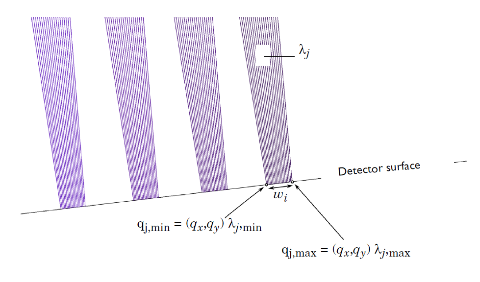
A zoomed-in view of the rays at the detector surface, illustrating how the width of the rays of a certain frequency are determined.
It is clear that rays of a single frequency are not focused to a single point. This naturally leads us to wonder about the resolution of the device. In other words, using the mirrors and grating as they are arranged in this model, what is the smallest change in wavelength that we can detect? It is possible to analyze the resolution using the Ray plot type. One way to quantify the resolution of the device is by using the expression
(3)
where S is the spectral width of the incident polychromatic beam, w_i is the width of an incident monochromatic beam at the detector, w_p is the width of a single pixel on the detector, and N is the total number of pixels. The resulting resolution is shown in the following plot.
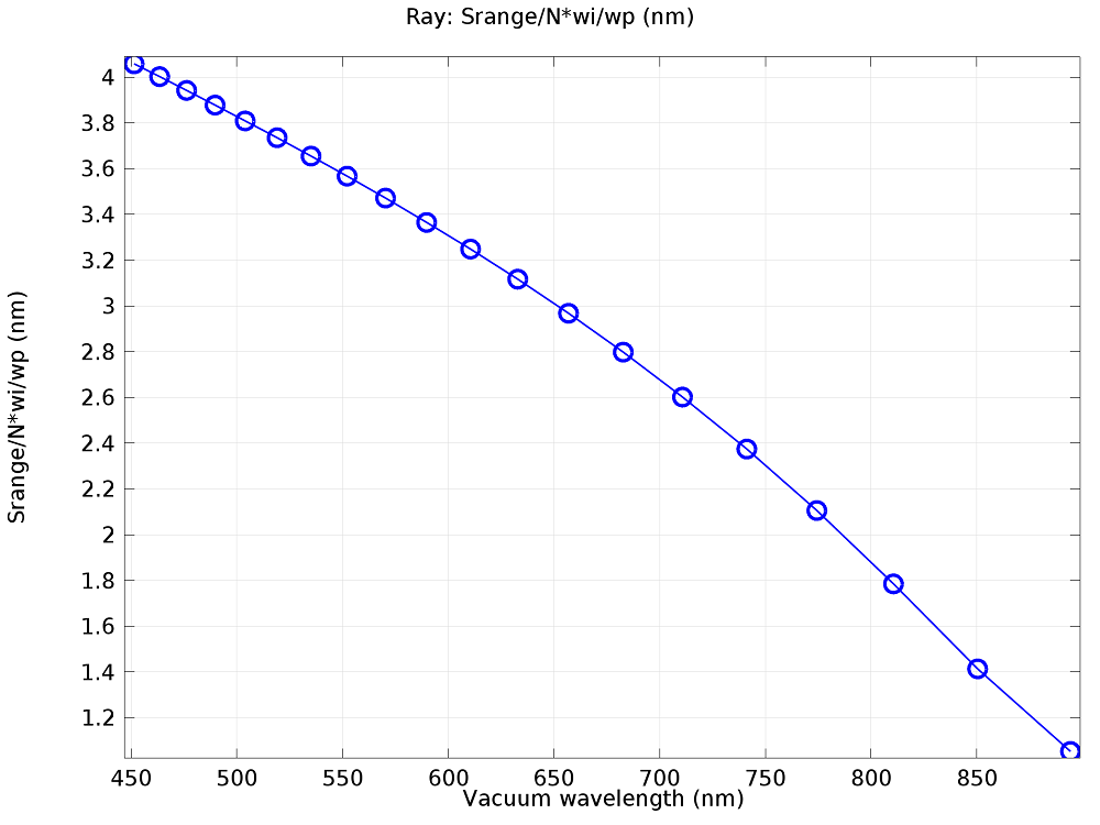
The spectral resolution of the Czerny–Turner monochromator as a function of the wavelength.
Modeling the Échelle Spectrometers
In the Ray Optics Module Application Library, you can find several complex 3D models of échelle spectrographs that are commonly used in astronomy for high-resolution analyses of stellar atmospheres and for precision Doppler velocimetry. In the White Pupil Échelle Spectrograph tutorial model, rays are traced through the fully parameterized geometry of a device and are focused by a Petzval lens. The échelle grating used in high order is defined via the grating blaze angle. The Cross Grating Échelle Spectrograph tutorial model demonstrates how to describe a periodic surface with two directions of periodicity via the Cross Grating feature.

The white pupil échelle spectrograph. The rays are colored according to their vacuum wavelength. To the right is an expanded view of the Petzval lens system, filtered so that only the axial rays for each wavelength are shown.
Next Step
To learn more about modeling the separation of polychromatic light with the Ray Optics Module, download the Czerny–Turner Monochromator model from our Application Gallery:

Comments (1)
Naif Alsalem
November 22, 2019Hi Chris,
Thank you for this nicely illustrated tutorial of CT spectrometer.
I would like to ask how did you determine the spectral range in the model? because what I see in the parameters table is one parameter named: Srange and its value is 650nm.
If I want to define my spectral range to be, for example, from 1700nm to 2300nm, how could I do this?
Thank you very much in advance
Best
Naif