In the previous installment of this series, we explained two concepts needed to model the release and propagation of real-world charged particle beams. We first introduced probability distribution functions in a purely mathematical sense and then discussed a specific type of distribution — the transverse phase space distribution of a charged particle beam in 2D. Now, let’s combine what we’ve learned and find out how to sample the initial positions and velocities of 3D beam particles from this distribution.
Reviewing 2D Phase Space Distributions and Ellipses
To start, let’s briefly review phase space distributions and ellipses in 2D, both of which are fully explained in the previous post in the Phase Space Distributions in Beam Physics series. The particles in real-world nonlaminar charged particle beams occupy a region in phase space that is often elliptical in shape. The equation for this phase space ellipse in 2D depends on the beam emittance ε and Twiss parameters,
(1)
where x and x’ are the transverse position and inclination angle of the particle, respectively. The Twiss parameters are further related by the Courant-Snyder condition,
(2)
The actual positions of particles in the ellipse can vary. Two of the most common distributions of phase space density are a uniform density within the ellipse and a Gaussian distribution with a maximum at the ellipse’s center, both of which are illustrated below. The blue curve in each case is the phase space ellipse described in Eq.(1), where ε is the 4-rms transverse emittance. For the Gaussian distribution, note that some particles still lie outside the ellipse. Since the Gaussian distribution decreases gradually without reaching exactly zero, there is always a chance that a few particles will lie outside the ellipse, no matter how large it is drawn. When using the 4-rms emittance to define the ellipse in Eq.(1), about 86% of the particles lie inside the ellipse.
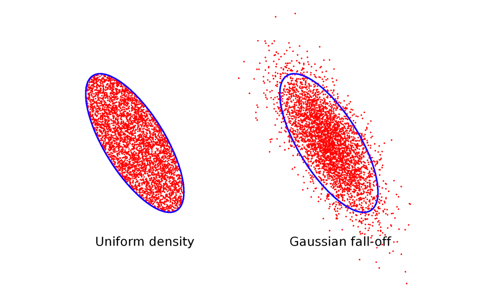
Comparison of a uniform and Gaussian distribution.
Let’s consider a simpler case in which the probability of finding a particle at any point in phase space is constant inside the ellipse and zero outside of it. For this problem, substituting Eq.(2) into Eq.(1) and solving for x’ yields
(3)
The probability distribution function is then
(4)
\begin{array}{cc}
C & -\frac{\alpha x}{\beta} -\frac{\sqrt{\varepsilon \beta -x^2}}{\beta} \textless x' \textless -\frac{\alpha x}{\beta} + \frac{\sqrt{\varepsilon \beta -x^2}}{\beta}\\
0 & \textrm{otherwise}
\end{array}\right.
where the constant C depends on the size of the ellipse. The probability g(x) of the particle having a given x-coordinate is
Considering the locations where Eq.(3) can take on real values, we get
\begin{array}{cc}
2C \frac{\sqrt{\varepsilon \beta -x^2}}{\beta} & -\sqrt{\varepsilon \beta} \textless x \textless \sqrt{\varepsilon \beta}\\
0 & \textrm{otherwise}
\end{array}\right.
Or, more simply,
(5)
Suppose we have a population of model particles that we want to sample using the probability distribution function given by Eq.(4). More specifically, we’d like to first sample the initial transverse positions of the particles according to Eq.(5) and then assign appropriate inclination angles so that the particles lie within the phase space ellipse. One way to accomplish this is to compute a cumulative distribution function starting from Eq.(5) and then use the method of inverse random sampling. Another possible method is using Eq.(5) to define the density of particles, which we can enter directly into the Inlet and Release features in the particle tracing interfaces. In this case, the normalization is done automatically.
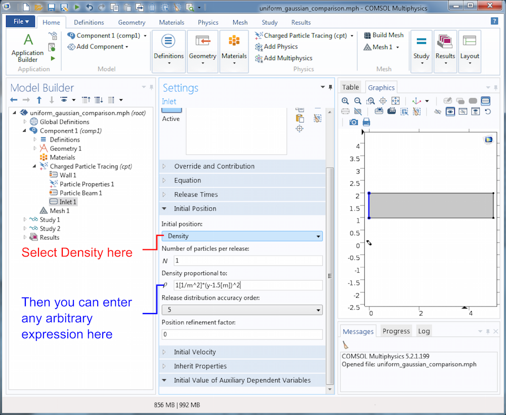
Screenshot showing how to input the particle density in the Inlet feature.
Still, the most convenient approach is using the Particle Beam feature available in the Charged Particle Tracing physics interface. The Particle Beam feature automatically distributes the particles in phase space, allowing you to specify the location of the beam center, emittance, and Twiss parameters.
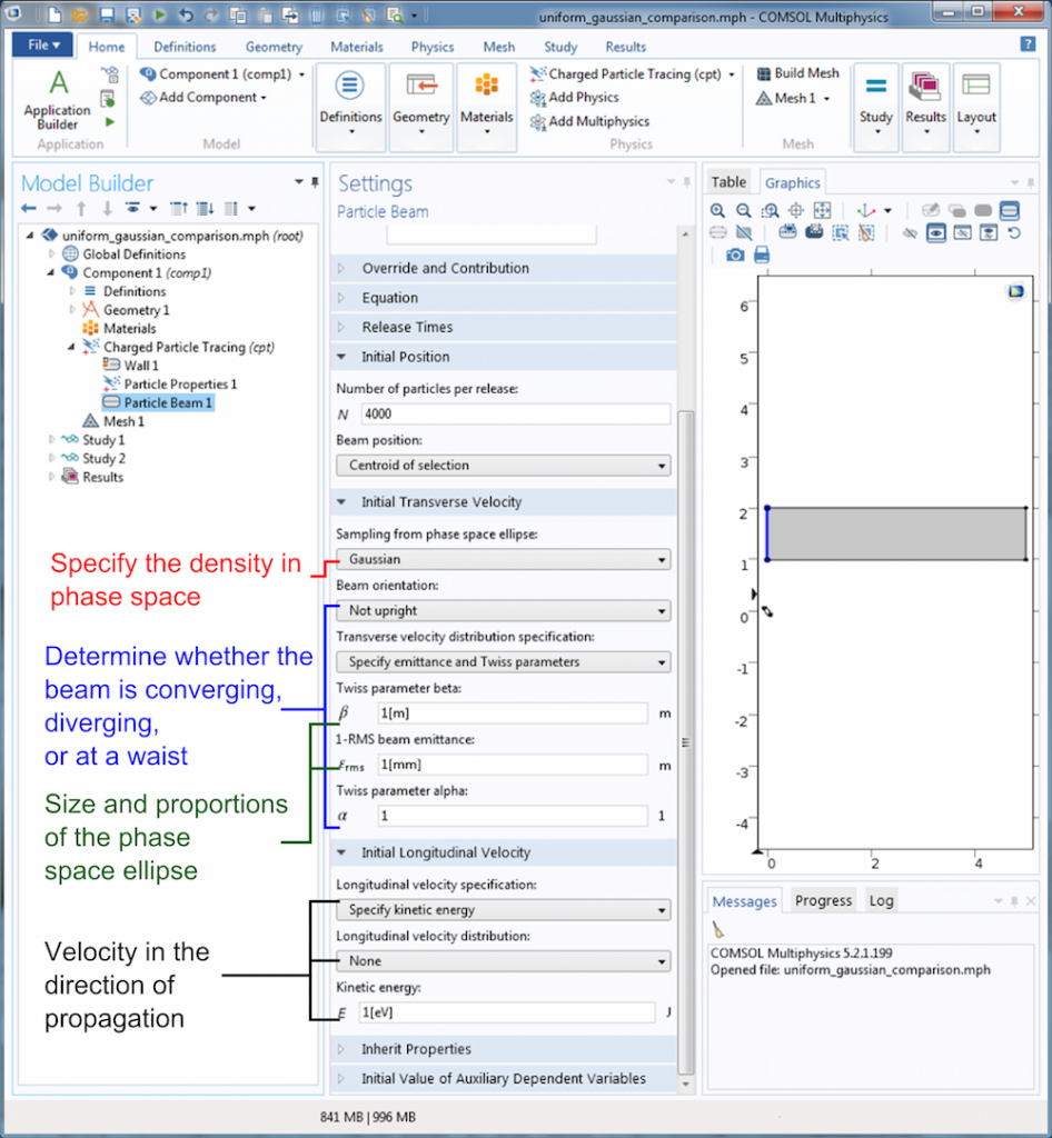
Screenshot showing how to input the particle density in the Particle Beam feature.
Simulating Charged Particle Beams in 3D
So far, we’ve only considered charged particle beams as idealized sheet beams where the out-of-plane (y) component of the transverse position and velocity can be ignored. However, real beams propagate in 3D space and only extend a finite distance in both transverse directions. Thus, in order to get a complete picture of a beam, we must consider two orthogonal transverse directions x and y as well as the inclination angles x' = v_x/ v_z and y' = v_y/v_z.
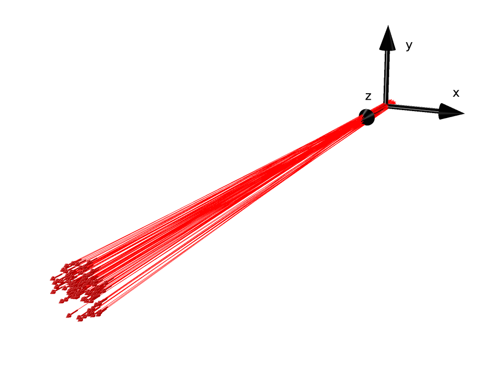
Particle beam propagating in 3D space.
The reason why simulating the release of particle beams in 3D is more complicated than in 2D is that the degrees of freedom for the two transverse directions are often coupled in real-world beams. For example, suppose two particles are released at the same transverse position i.e., the same x– and y-coordinates. Let’s say that one of these particles has a very large inclination angle in the x direction (x’) and the other particle has a very small inclination angle in the x direction. The particle with the large inclination angle in the x direction is more likely to have a small inclination angle in the y direction and vice versa. Hence, we can’t just sample from two different distributions for x’ and y’ because the value of each one affects the probability distribution of the other.
To phrase this problem in a more abstract sense: Instead of considering the two transverse directions as separate 2D phase space ellipses, we actually need to think about the transverse particle motion using distributions of phase space in four dimensions! Since we’re used to seeing objects only in 2D or 3D, distributions with more than three space dimensions are much harder to visualize.
This is where the Particle Beam feature is most useful. It includes settings for sampling the initial particle positions and inclination angles from a variety of built-in 4D transverse phase space distributions. Some common distributions are the Kapchinskij-Vladimirskij (KV) distribution, waterbag distribution, parabolic distribution, and Gaussian distribution. First, let’s consider the simplest distribution, the KV distribution, and then visualize the other distributions in this group.
Mathematically, the KV distribution considers the beam particles to be uniformly distributed on an infinitesimally thin, 4D hyperellipsoid in phase space. It’s written as
+\left(\frac{r_x x' -r'_x x}{\varepsilon_x} \right)^2
+\left(\frac{y}{r_y} \right)^2
+\left(\frac{r_y y' -r'_y y}{\varepsilon_y} \right)^2 = 1
where rx and ry are the maximum extents of the beam in the x and y directions, εx and εy are the beam emittances associated with the two transverse directions, and r’x and r’y are the inclination angles at the edge of the beam envelope.
Because it is more difficult to visualize 4D probability distribution functions than functions of lower dimensions, it is often convenient to visualize the distribution indirectly by plotting its projection onto lower dimensions. An interesting property of the KV distribution is that its projection onto any 2D plane is an ellipse of uniform density. The projections onto six such planes are shown below. The projections of the 4D hyperellipsoid onto the x-x’ and y-y’ planes are tilted because nonzero values have been specified for the Twiss parameter α in each transverse direction.
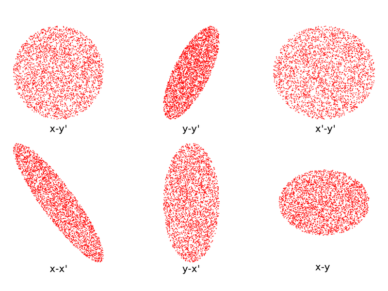
The KV distribution projected onto six 2D planes.
Compare the distributions shown above to the following alternatives.


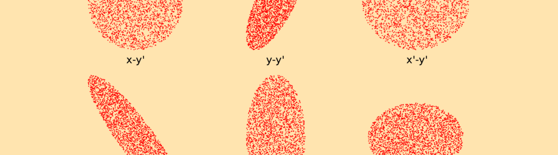
The waterbag, parabolic, and Gaussian distributions projected onto six 2D planes.
We see that the projection onto any 2D plane forms an ellipse-shaped distribution in all cases, but the ellipses are only uniformly filled in the KV distribution.
Concluding Thoughts on Modeling Charged Particle Beams
Even as this blog series on modeling charged particle beams comes to a close, we have only scratched the surface of the intricate and highly technical field of beam physics. While we’ve discussed transverse phase space distributions in 3D, we haven’t examined longitudinal emittance or the related phenomenon of bunching. We also haven’t categorized the phenomena that causes emittance to increase, decrease, or remain constant as the beam propagates.
This series is meant to be an introduction to the way in which random or pseudorandom sampling from probability distribution functions plays an important role in capturing the real-world physics of high-energy ion and electron beams. For a more comprehensive overview of beam physics, references 1-3 provide an excellent starting point. More technical details about each of the 4D transverse phase space distributions described above, including algorithms for sampling pseudorandom numbers from these distributions, can be found in references 4-7. To learn more about how these concepts apply in the COMSOL Multiphysics® software, browse the resources featured below or contact us for guidance.
Other Posts in This Series
- Sampling Random Numbers from Probability Distribution Functions
- Phase Space Distributions and Emittance in 2D Charged Particle Beams
References
- Humphries, Stanley. Principles of charged particle acceleration. Courier Corporation, 2013.
- Humphries, Stanley. Charged particle beams. Courier Corporation, 2013.
- Davidson, Ronald C., and Hong Qin. Physics of intense charged particle beams in high energy accelerators. Imperial college press, 2001.
- Lund, Steven M., Takashi Kikuchi, and Ronald C. Davidson. “Generation of initial Vlasov distributions for simulation of charged particle beams with high space-charge intensity.” Physical Review Special Topics — Accelerators and Beams, vol. 12, N/A, November 19, 2009, pp. 114801 12, no. UCRL-JRNL-229998 (2007).
- Lund, Steven M., Takashi Kikuchi, and Ronald C. Davidson. “Generation of initial kinetic distributions for simulation of long-pulse charged particle beams with high space-charge intensity.” Physical Review Special Topics — Accelerators and Beams, 12, no. 11 (2009): 114801.
- Batygin, Y. K. “Particle distribution generator in 4D phase space.” Computational Accelerator Physics, vol. 297, no. 1, pp. 419-426. AIP Publishing, 1993.
- Batygin, Y. K. “Particle-in-cell code BEAMPATH for beam dynamics simulations in linear accelerators and beamlines.” Nuclear Instruments and Methods in Physics Research. Section A: Accelerators, Spectrometers, Detectors and Associated Equipment 539, no. 3 (2005): 455-489.


Comments (0)