

In order to ensure safe geotechnical building methods, specific applications require certain foundations and structure reinforcements. Tests are quite expensive to carry out, so simulation can be really useful and even essential. Many numerical models have been developed to give a deep insight into soil behavior. Here, we introduce the most widespread models for soils available in COMSOL Multiphysics and analyze a tunnel excavation example.
Quick Note on Geotechnical Engineering
There seems to be a general trend when it comes to construction. Offshore structures are constructed in deeper and deeper waters; buildings are constructed increasingly close to each other; offshore wind turbines are developed in deep waters far away from the coasts, which are likely to experience extreme loading conditions. Therefore, in recent decades, geotechnical engineers have developed numerical simulations to cope with this construction trend and ensure safe building methods.
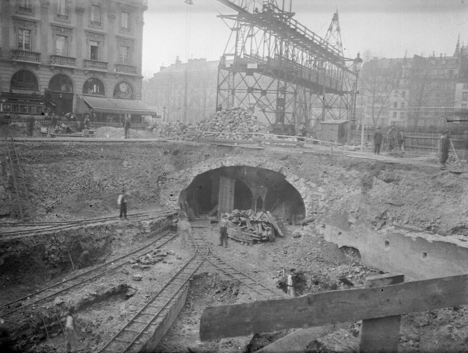
“Paris Metro construction 03300288-3”. Licensed under Public domain via Wikimedia Commons.
Plasticity and Geomaterials
Materials for which strains or stresses are not released upon unloading are said to behave plastically. Several materials behave in such a manner, including metals, soils, rocks, and concrete, for example. These give rise to an elastic behavior up to a certain level of stress, the yield stress, at which plastic deformation starts to occur.
The elastic-plastic behavior is path-dependent and the stress depends on the history of deformation. Therefore, the plasticity models are usually written connecting the rates of stress, rather than stress, and the plastic strain. The most widespread and well-known plasticity model throughout the industry is based on the von Mises yield surface for which plastic flow is not altered by pressure. Therefore, the yield condition and the plastic flow are only based on the deviatoric part of the stress tensor.
However, this model is no longer valid for soil materials since frictional and dilatation effects need to be taken into account. Let’s see how this can be worked out and briefly explain the different soil plasticity models available in the COMSOL Multiphysics® simulation software.
Plasticity of Soils and Rocks
For materials such as soils and rocks, the frictional and dilatational effects cannot be neglected. This whole class of materials is well known to be sensitive to pressure, leading to different tensile and compressive behaviors. The von Mises model presented above is thus not suitable for these types of materials. Instead, yield functions have been worked out to take into account the behavior of frictional materials.
Let’s illustrate the frictional behavior and plastic flow for these materials by considering the block shown here:
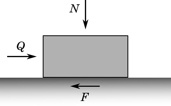
The block is loaded as shown by a normal load N and a tangential load Q. Assuming that the block rests on a surface with a coefficient of static friction \mu, according to Coulomb’s law, the maximum force that the block can withstand before sliding is given by F=\mu N. Therefore, the onset of sliding occurs when the following condition is reached:
(1)
The direction of sliding is horizontal. For tangential loads such as f<0, the block will not slide, but as soon as f=0, the block will slide in the direction of the applied load Q. The Mohr-Coulomb criterion — the first soil plasticity model ever developed — is a generalization of this approach to continuous materials and a multiaxial state of stress. It is defined such that yielding and even rupture occur when a critical condition that combines the shear stress and the mean normal stress is reached on any plane. This condition is stated as below:
(2)
Here, \tau is the shear stress, \sigma is the normal stress, c is the cohesion representing the shear strength under zero normal stress, and \mu=\tan\phi is the coefficient of internal friction coming from the well-known Coulomb model of friction. This equation represents two straight lines in the Mohr plane. A state of stress is safe if all three Mohr’s circles lie between those lines, while it is a critical state (onset of yielding) if one of the three circles is tangent to the lines.
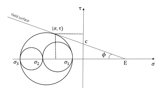
Mohr-Coulomb yield behavior. The Mohr circles are based on the principal stresses \sigma_1, \sigma_2, and \sigma_3. As you can see, one of the circles is tangential to the yield surface, and so the onset of yielding is occurring.
According to the figure above, the stress state is given by \tau=\frac{1}{2}(\sigma_1-\sigma_3)\cos\phi and \sigma=\frac{1}{2}(\sigma_1+\sigma_3)+\frac{1}{2}(\sigma_1-\sigma_3)\sin \phi. The yield criterion and Equation 2 can therefore be re-written in a generalized form as follows:
(3)
It can even be seen as a particular case of a more general family of criteria based on Coulomb friction and written by equations based on invariants of the stress tensor:
(4)
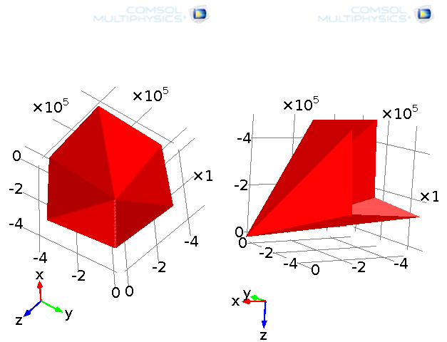
Representation of the Mohr-Coulomb yield function.
The Mohr-Coulomb criterion defines a hexagonal pyramid in the space of principal stresses, which makes it straightforward for this criterion to be treated analytically. But, the constitutive equations are difficult to handle from a numerical point of view because of the sharp corners (for instance, the normal of this yield surface is undefined at the corners).
In order to avoid the issue associated with the sharp corners, another yield criterion of this family, the Drucker–Prager yield criterion, has been developed by modifying the von Mises yield criterion to take into account the Coulomb friction, i.e., incorporate a hydrostatic pressure dependency:
(5)
This represents a smooth circular cone in the plane of principal stress, rather than a hexagonal pyramid. If the coefficients \alpha and k are chosen such that they match the coefficients in the Mohr-Coulomb criterion, as follows:
(6)
the Drucker–Prager yield surface passes through the inner or outer apexes of the Mohr-Coulomb pyramid, depending on whether the symbol \pm is positive or negative. The plastic flow direction is taken from the so-called “plastic potential”, which can be either the same, associative plasticity, or different, non-associative plasticity, than the onset of yielding (the yield function). Many different non-associative flow rules can be developed.
Using an associative law for the Drucker–Prager model leads the volumetric plastic flow to be nonzero. Therefore, there is a change in volume under compression. However, this is contradictory to the behavior of many soil materials, particularly granular materials. Instead, a non-associative flow rule can be used such that the plastic behavior is isochoric (volume preserving) — a much better reflection of the plastic behavior of granular materials.
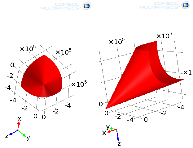
Representation of the Drucker–Prager yield function.
Non-Associative Law for Soil Plasticity in COMSOL Multiphysics
Next, I will show you how to use a non-associative law for soil plasticity in COMSOL Multiphysics. Non-associative plastic laws can be used regardless of the plasticity model used in the software.
If you’re using the Mohr-Coulomb model, there are basically two different approaches to handling non-associative plasticity. The plastic potential can either be taken from the Drucker–Prager model or be the same as the Mohr-Coulomb yield function but with a different slope with respect to the hydrostatic axis, i.e., the angle of friction is replaced by the dilatation angle (see screenshot below).
Moreover, when using the Drucker–Prager matched to a Mohr-Coulomb criterion, it is easy to adapt the dilatation angle to match with the non-associative law that you want to use. For instance, the non-associative law presented above can be worked out by taking the dilatation angle null.
Last but not least, a useful feature called elliptic cap has been developed to avoid unphysical behavior of the material beyond a certain level of pressure. Indeed, real-life material cannot withstand infinite pressure and still deform elastically. Therefore, to cope with this, we can use the elliptic cap feature available in COMSOL Multiphysics.
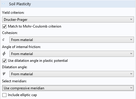
Soil Plasticity feature settings window.
Let’s try to put into practice everything we’ve learned so far by analyzing the example of a tunnel excavation. This will also be an opportunity to figure out what the effects of the different features we mentioned above are.
Example of a Tunnel Excavation
The simulation of a tunnel excavation process is especially important in predicting the necessary reinforcements that the workers need to use to avoid the collapse of the construction.
The following model aims to simulate the soil behavior during a tunnel excavation. The surface settlement (i.e., the vertical displacement along the free ground surface) and the plastic region are computed and compared between the different soil models used to carry out this simulation. The geometry we’ll use is presented in the figure below. To make our model realistic, infinite elements have been used to enlarge the soil domain, while keeping the computational domain small enough to get the solution in a relatively short time.
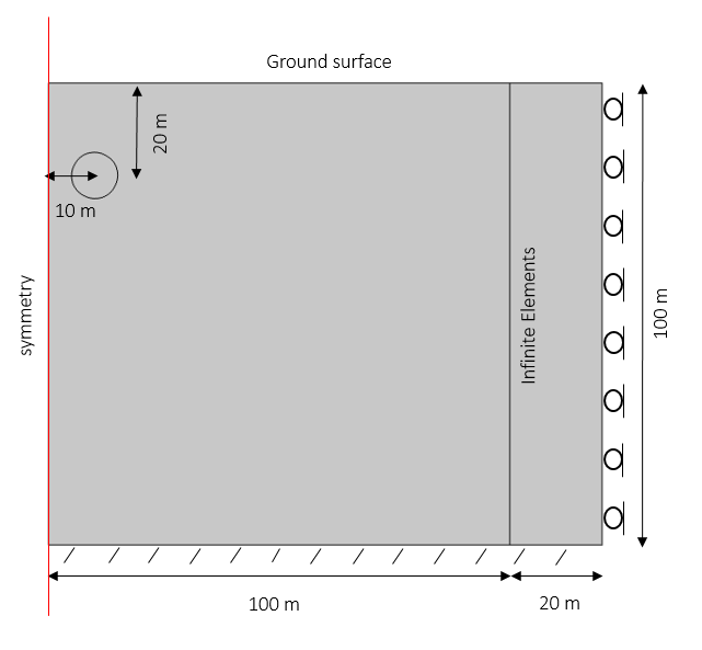
The geometry consists of a soil layer that is 100 meters deep and 100 meters wide plus 20 meters of infinite elements. A tunnel 10 meters in diameter is placed 10 meters away from the symmetry axis and 20 meters below the surface.
First of all, we need to add the in-situ stresses in the soil before the excavation of the tunnel. Then, we can compute the elastoplastic behavior once the soil corresponding to the tunnel is removed. The in-situ stresses must be incorporated in this second step. This is fairly straightforward to set up in COMSOL Multiphysics.
We can begin by adding a stationary step where the in-situ stresses will be computed. Then, in a second step but still within the same study, we add a soil plasticity feature. Finally, we compute the solution. In order to get the pre-stresses incorporated into the second step, we should add an Initial Stress and Strain feature under the Solid Mechanics interface, as shown below.
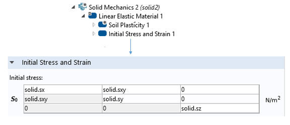
Initial Stress and Strain feature used to incorporate the in-situ stresses from the first step as initial stresses for the second step, during which excavation occurs. The variables solid.sx, solid.sxy, etc. are the x-components of the stress tensor, the xy-components of the stress tensor, etc.
The first plot shows the in-situ stresses computed from the first step. These stresses result from the gravity load.
The von Mises stress in the soil before the excavation of the tunnel.
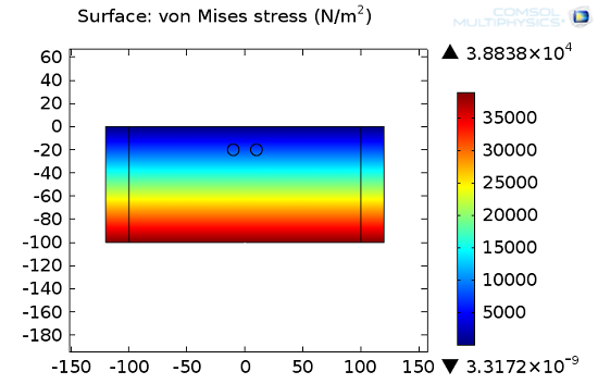
The second plot shows the stress distribution after excavating the tunnel. In-situ stresses are taken from the first step. Note, as expected, the increase in the von Mises stress around the tunnel as well as the deformation of the tunnel shape.
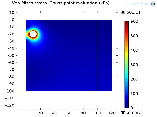
The von Mises stress in the soil after excavation of the tunnel.
As mentioned previously, while removing the tunnel domain, a plasticity feature is added and the soil experiences a plastic behavior. This is depicted in the figure below of a Drucker–Prager model with associative plastic flow. The plastic region is concentrated around the near surroundings of the tunnel. The analysis of this region is quite important in gaining insight into how the soil is more likely to deform. Therefore, it allows us to handle the necessary reinforcements in order to avoid collapse and get the desired tunnel shape.
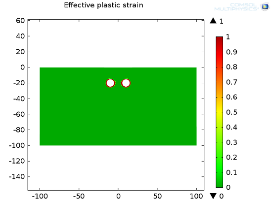
Plastic region after excavating the tunnel.
This tunnel excavation simulation has been carried out in four different cases in order to compare the different soil models presented in the previous section as well as understand the influence of the cohesion on the soil’s behavior. The results are shown by taking the surface settlement as the criterion.
Below, we have a 1D plot from which we can observe the following relationship: The lower the cohesion, the greater the deformation. We can also note that the Mohr-Coulomb model tends to, somehow, make the soil stiffer than the Drucker–Prager model. The non-associative law with a null dilatation angle prevents the soil from dilating under compression and so the surface settlement becomes greater.
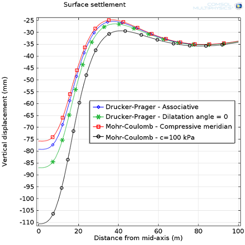
Surface settlement comparison between different plasticity models and material properties.
Further Reading
There are also a couple of other plasticity models for soil, rocks, and concrete available in COMSOL Multiphysics. Please check out the links below to get further information about geotechnical simulations and the Geomechanics Module of COMSOL Multiphysics.
Also, be sure to watch the video on how to build a model of an excavation:

Comments (1)
Shashank Tiwari
July 19, 2018Hello:
In this model, the in-situ stresses are initialized with the “Initial Stress” option as shown in one of the images above. Could you please suggest if the input value of the initial strain will be 0 or it needs be incorporated?
I look forward to hearing your comment.
Thanks,
Shashank