

In the latest post in this Hybrid Modeling blog series, we discussed the basic principles behind shared memory computing — what it is, why we use it, and how the COMSOL software uses it in its computations. Today, we are going to discuss the other building block of hybrid parallel computing: distributed memory computing.
Processes and Clusters
Recalling what we learned in the last blog post, we now know that shared memory computing is the utilization of threads to split up the work in a program into several smaller work units that can run in parallel within a node. These threads share access to a certain portion of memory — hence the name shared memory computing. By contrast, the parallelization in distributed memory computing is done via several processes executing multiple threads, each with a private space of memory that the other processes cannot access. All these processes, distributed across several computers, processors, and/or multiple cores, are the small parts that together build up a parallel program in the distributed memory approach.
To put it plainly, the memory is not shared anymore, it is distributed (check out the diagram in our first blog post in this series.)
To understand why distributed computing was developed in this way, we need to consider the basic concept of cluster computing. The memory and computing power of a single computer is limited by its resources. In order to get more performance and to increase the amount of available memory, scientists started connecting several computers together into what is called a computer cluster.
Splitting of the Problem
The idea of physically distributing processes across a computer cluster results in a new level of complexity when parallelizing problems. Every problem needs to be split into pieces — the data needs to be split and the corresponding tasks need to be distributed. Consider a matrix type problem, where operations are performed on a huge array. This array can be split into blocks (maybe disjointed, maybe overlapping) and each process then handles its private block. Of course, the operations and data on each block might be coupled to the operations and data on other blocks, which makes it necessary to introduce a communication mechanism between the processes.
To this end, data or information required by other processes will be gathered into chunks that are then exchanged between processes by sending messages. This approach is called message-passing, and messages can be exchanged globally (all-to-all, all-to-one, one-to-all) or point-to-point (one sending process, one receiving process). Depending on the couplings of the overall problem, a lot of communication might be necessary.
The objective is to keep data and operations as local as possible in order to keep the communication volume as low as possible.
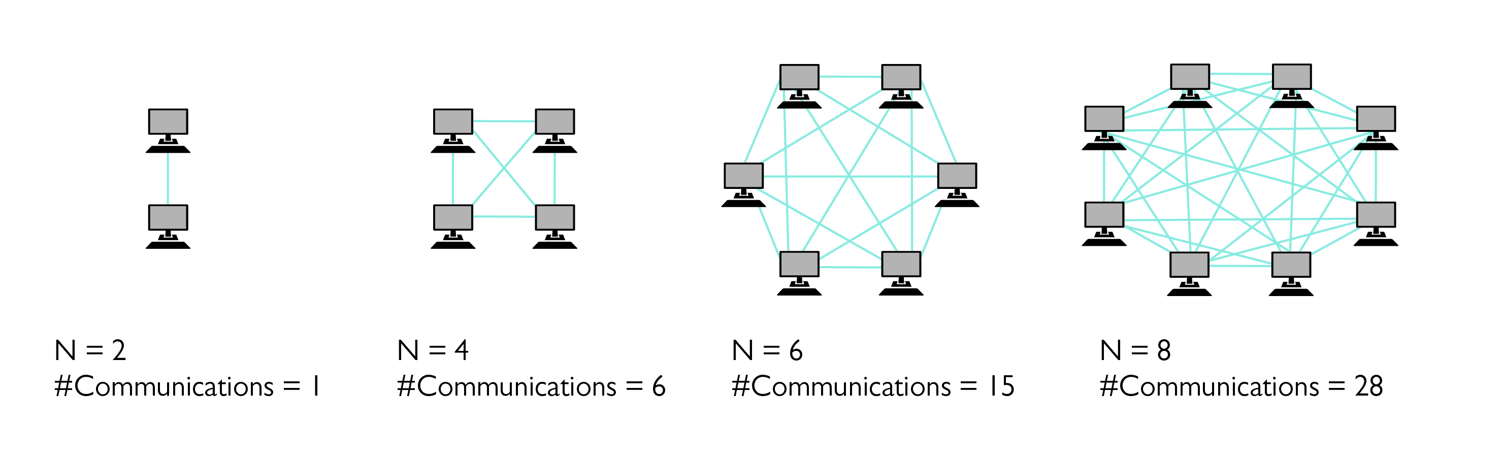
The number of messages that needs to be sent in all-to-all can be described by a complete graph. The increase is quadratic with respect to the number of compute nodes used.
Speeding up Computations or Solving Larger Problems
The scientist who is working on a computer cluster can benefit from the additional resources in the following two ways.
First, with more memory and more computing power available, she can increase the problem size and hereby solve larger problems in the same amount of time through adding additional processes and keeping the work load per process (i.e. size of the subproblem and number of operations) at the same level. This is called weak scaling.
Alternatively, she can maintain the overall problem size and distribute smaller subproblems to a larger number of processes. Every process then needs to deal with a smaller workload and can finish its tasks much faster. In the optimal case, the reduction in computing time for a problem of fixed size distributed on P processes will be P. Instead of one simulation per time unit (one hour, one day, etc.), P simulations can be run per time unit. This approach is known as strong scaling.
In short, distributed memory computing can help you solve larger problems within the same amount of time or help you solve problems of fixed size in a shorter amount of time.
Communication Needed
Let’s now take a closer look at message-passing. How do the processes know what the other parts of the programs are doing? As we know from above, the processes explicitly have to send and receive the information and variables that they or other processors need. This, in turn, brings with it some drawbacks, especially concerning the time it takes to send the messages over the network.
As an illustration, we can recall the conference room analogy discussed in the shared memory blog post, where collaborative work occurred around a table and all the information was made freely available for everyone sitting at that table to access and work in, even in parallel. Suppose that this time, the conference room and its table have been replaced by individual offices, where the employees sit and make changes to the papers they have in front of them.
In this scenario, one employee, let’s call her Alice, makes a change to report A, and wants to alert and pass these changes to her coworker Bob. She now needs to stop what she’s doing, get out of her office, walk over to Bob’s office, deliver the new information, and then return to her desk before continuing to work. This is much more cumbersome than sliding a sheet of paper across the table in a conference room. The worst case in this scenario is that Alice will spend more time alerting her coworkers about her changes than actually making changes.
The communication step in the new version of our analogy can be a bottleneck, slowing down the overall work progress. If we were to reduce the amount of communication that needs to be done (or speed up the communication, perhaps by installing telephones in the offices, or using an even faster kind of network) we could spend less time waiting on messages being delivered and more time computing our numerical simulations. In distributed memory computing, the bottleneck is usually the technology that passes electronic data to each other, the wires between the nodes, if you like. The current industry standard for providing high throughput and low latency is Infiniband, which allows the passage of messages to occur a lot quicker than ethernet.
Why Use Distributed Memory?
Distributed memory computing has a number of advantages. One of the reasons why you would utilize distributed memory is the same as in the shared memory case. When adding more compute power, either in the form of additional cores, sockets, or nodes in a cluster, we can start more and more processes and take advantage of the added resources. We can use the gained compute power to get the results of the simulations faster.
With the distributed memory approach, we also get the advantage that with every compute node added to a cluster, we have more memory available. We are no longer limited by the amount of memory our mainboard allows us to build in and we can, in theory, compute arbitrarily large models. In most cases, scalability of distributed memory computing exceeds that of shared memory computing, i.e. the speed-up will saturate at a much larger number of processes (compared to the number of threads used).

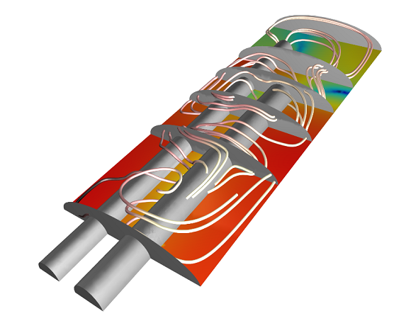
Number of simulations per day with respect to the number of processes used for the Perforated Muffler model depicted below. A 1 GB/s ethernet was used as the communication network. The first four processes are executed on one compute node, and the ethernet network comes into use after that. The small difference in simulations per day between 4 and 5 processes shows the impact of a slow communications network, even for a parametric problem. The compute nodes used are equipped with Intel® Xeon® E5-2609 and 64 GB DDR3 @1600 MHz.
However, we do have to be aware of the limitations as well. Just as in the shared memory case, there are some problems that are well suited for computing with the distributed memory approach, while others are not. This time, we also need to look at the amount of communication that is needed to solve the problem, not only if it is easily parallelized.
Consider, for instance, a time-dependent problem where a large amount of particles are interacting in such a way that after each step, all of the particles need to have the information about every other particle. Assuming that each of the particles are computed by its own process, the amount of communications in such an example can be described by the fully connected graphs (shown above), and the number of messages per iteration grows rapidly as the number of particles and processes increase. In contrast, a parametric sweep, where the parametric values can be computed independently of each other, requires almost no communication at all, and will not suffer as much from the communication bottleneck.
The model for which the speed-up was obtained. It is a small parametric model (750,000 degrees of freedom) using the PARDISO direct solver. This model is available in the Model Gallery.
How COMSOL Takes Advantage of Distributed Memory Computing
Users that have access to a floating network license (FNL) have the possibility to use the distributed functionality of the COMSOL software on single machines with multiple cores, on a cluster, or even in the cloud. The COMSOL software’s solvers can be used in distributed mode without any further configuration. Hence, you can do larger simulations in the same amount of time or speed up your fixed-size simulation. Either way, COMSOL Multiphysics helps you to increase your productivity.
The distributed functionality is also very useful if you are computing parametric sweeps. In this case, you can automatically distribute the runs associated to different parameter values across the processes you are starting COMSOL Multiphysics with. Since the different runs in such a sweep can be computed independently of each other, this is called an “embarrassingly parallel problem”. The speed-up is, with a good interconnection network, almost the same as the number of processes.
For a detailed instruction on how to set up your compute job for distributed memory computing, we recommend the COMSOL Reference manual, where we list several examples on how to start COMSOL in distributed mode. You may also refer to the user guide of your HPC cluster for details about how to submit computing jobs.
Next up in this blog series, we will dig deeper into the concept of hybrid modeling — check back soon!

Comments (2)
Daniel McLean
February 20, 2014It seems to me that the # Communications links on your first page for an arrangement with n=8 nodes is incorrect. It should be 28, i.e. Sum of 1 to n-1.
Fanny Littmarck
February 20, 2014Thanks for pointing out this typo, Daniel. The image has been updated.