
A lot of effort is put into inventing or improving existing technologies used to cool buildings, food, or any goods that need to be stored at a definite temperature. The reason is simple: adopting more efficient designs will result in achieving the same goal while consuming less energy. Both our balance sheet and the environment will benefit from these solutions. Here we will explore modeling temperature of a passive cooling design using a wine cellar as an example.
Active or Passive Cooling?
When dealing with cooling, the first decision to make is: active or passive? If we go for an active cooling technology, then we have to rely on mechanical components. Such a solution is not “green” and usually results in high operating costs. What if we opt for a passive cooling method instead? In this case our knowledge of physics will help us satisfy our cooling needs without energy-consuming components. A good example of how to apply the principles of physics to implement a passive cooling technology is the design of “green” buildings. Another example that I’m sure you will find interesting is wine cellars, where the thermal properties of the ground surrounding the cellar help mitigate the variations in temperature from the outside environment.
Keeping a Wine Cellar Cool
Active cooling applied to wine storage is pretty simple. You can think of it as a bigger version of a refrigerator. Simulation can help a lot in achieving an efficient design where, basically, if we have enough power, we can make our cooling system work even if the size of the storage or the distribution of the wine racks is not optimal.
What I believe is more challenging (and fun!) than an active cooled cellar is the design of a passive cooled cellar. It’s true that its operating costing costs are very low and its performance doesn’t depend on external sources of energy, like electricity. Yet, its design needs to satisfy several constraints that are not set by us. In order to succeed, we have to answer questions like: Given certain thermal properties of the ground, or a location subject to a certain kind of climate, how deep should I dig for my cellar for it to work? How big should it be? Where should I put my wine racks?
When simulation wasn’t so fast, accurate, and easy to perform as it is today, the construction of a passive cooled cellar relied a lot on experience. I’m sure that more than a few of them were too cold or too warm (wine should be stored around 12°C and deviations from this value shouldn’t exceed ±2°C). Digging deeper, or reducing the depth of the cellar once it’s already been built and operating, must have been expensive.
Modeling Temperature: Passive Cooling of a Wine Cellar
Today we can easily set up a simulation and find the optimal cellar’s depth given the thermal properties of the ground and the variation of temperature above it as a function of time. In Figure 1, I’ve depicted the computational domain. As you can see, I’ve opted for a 2D axisymmetric simulation and used an infinite element domain to reduce the size of the simulation without sacrificing its accuracy. In other words an infinite element domain is a domain that is mathematically stretched out towards infinity. We don’t have to worry about implementing such a fantastic technology; COMSOL Multiphysics will take care of it for us under the hood.
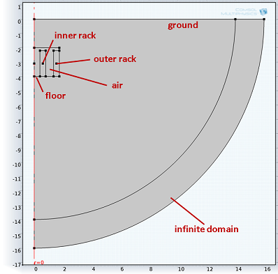
Figure 1. Domains used for the simulation. The simulation is 2D axisymmetric.
I positioned the cellar at a depth of 2 m, added wine racks (I assumed their thermal properties to be the same as water), included the air (which is a good insulator) present in the cellar, and assigned an initial temperature of 12°C. As a boundary condition at the surface of the ground, I used the expression Tground = Taverage + ΔT · cos(ω · t) where Tground = 12°C, ΔT = 20°C, and ω = 2 · π · ƒ = 2 · π/P with P = 365 days.
It’s interesting to see from the results shown in Figure 2 that the thermal properties of the ground and the depth and geometry of the cellar enable the dampening of the heat wave originating from the surface of the ground. In this case, both the thermal properties and the depth are optimal. The initial value of 12°C doesn’t vary more than 3°C. This design can be accepted by most wine buffs and can be further refined by running a simulation where different depths and cellar configurations are explored.
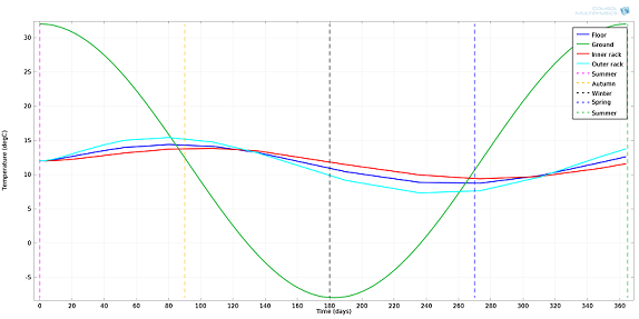
Figure 2. Temperature as a function of time in different points of the computational domain.
Below you can see a 3D representation of the temperature field after 1 year (the temperature in the infinite element domain is not shown). We can note that at the height of summer the temperature of the cellar is still acceptable, with the ground and air helping greatly to insulate it.
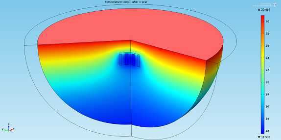
Figure 3. Temperature distribution in the computational domain after 1 year.
Figure 4 below depicts the temperature profile along the axis of symmetry with the cellar placed between 2 m and 4 m below the surface of the ground. This is one of my favorite plots since it allows us to really “see” the thermal dampening effect of the ground surrounding the cellar and capture the temperature inversion that occurs during the summer and winter. Pretty neat, wouldn’t you say?
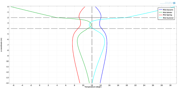
Figure 4. Temperature profile as a function of depth along the axis of symmetry r=0 (see Figure 1). The vertical dashed line represents the average temperature of ≈12°C. The two horizontal dashed lines represent the ceiling (z=-2 m) and the floor (z=-4 m) of the cellar, respectively. The four solid lines represent the temperature profile for different seasonal points. Profiles are not symmetrical around the average temperature due to the damped wave nature of the solution.
As you’ve seen here, by modeling temperature virtually, it’s not only possible to design our own passive cooled wine cellar, but it’s relatively easy, too.





Comments (0)