
Guest blogger Linus Fagerberg from Lightness by Design returns to share a novel approach for predicting external noise generation in muffler designs.
In recent years, the European Union has introduced stricter noise emission limits for road vehicles. For those designing mufflers, these limits make it important to create more efficient ways of developing and assessing the performance of their designs. At Lightness by Design, we’ve developed a novel approach that accomplishes this goal.
Building on a Previous Muffler Model
A 2016 blog post illustrates the impact of including structural effects in a pure acoustics model through the use of an automotive muffler geometry in the COMSOL Multiphysics® software. The effect on the predicted transmission loss for the muffler modeled with pure pressure acoustics was compared with the multiphysics model.
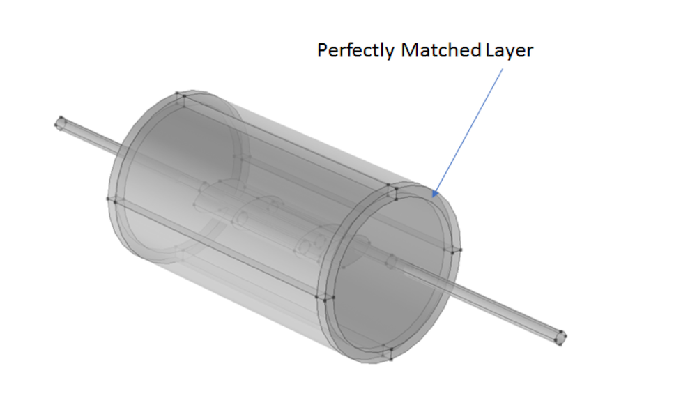
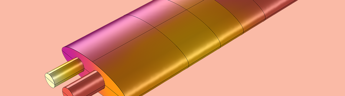
Figure 1. The muffler model contained in the acoustic domain with a surrounding perfectly matched layer.
Lightness by Design has extended the acoustic-structure coupling for the muffler model to evaluate the sound leakage from the muffler into the surrounding atmosphere. To facilitate this evaluation, a cylinder-shaped acoustic domain with a radius of 0.35 m and length of 1.4 m is added to encompass the muffler, with the domain’s center placed at the center of the muffler (shown in Figure 1). The external domain layer, with a thickness of 50 mm, enables the definition of a perfectly matched layer (PML), which represents a nonreflecting condition.
Modeling the Muffler Design in COMSOL Multiphysics®
Muffler geometry similitude is retained from the previous study and material properties and boundary conditions applied to the muffler geometry are kept as well. Therefore, the surfaces of the extruded inlet and outlet pipe sections of the muffler going through the acoustic domain are modeled as sound hard boundaries, as indicated in the image below. A Plane Wave Radiation boundary condition is applied at both ends of the pipe and a 1 Pa incident plane wave is applied at the inlet face of the muffler. For a visual description, see Figure 2.
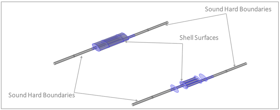
Figure 2. The muffler model showing the applied boundary conditions.
The acoustic domain is modeled with the acoustic properties of air at an ambient temperature of 20°C. These properties are identical to the acoustic properties of air inside the muffler volume.
The Plane Wave Radiation condition introduces the artificial damping of any outgoing pressure waves (to minimize the reflection), thus replicating an unbounded or “infinite” pipe. The same mesh size settings, as defined and applied to the muffler geometry in the previous study, are applied to the muffler and acoustic domains of interest here. The external PML region is swept with six elements through the thickness. The acoustic-shell multiphysics coupling has a similar setup to the one in the prior study.
Defining the Transmission Loss
The transmission loss is a good quantity by which to gauge the performance of a muffler. The transmission loss, TL, from the muffler inlet to the muffler outlet was defined in the previous study as:
where Pin is the acoustic power at the muffler inlet and Pout is the acoustic power at the muffler outlet.
For the model at hand, not only is the transmission loss from the inlet of the muffler to the outlet of the muffler of interest, but also the transmission loss from the inlet of the muffler to the boundary of the acoustic domain is also important to evaluate (Figure 3 indicates these boundaries). The latter provides a means to numerically evaluate the sound leakage from the muffler into the surrounding atmosphere. The radiated power is found by integrating the acoustic intensity on the exterior physical surface (on the inside of the PML).
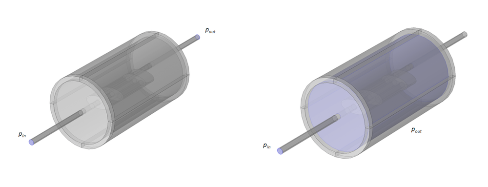
Figure 3. The muffler model and acoustic domain. The boundaries included in the transmission loss calculation are shown.
Comparing the Simulation Results for the Transmission Loss in a Muffler
A harmonic analysis for a frequency range of 10 to 750 Hz and a shell thickness of 1 mm has been conducted for the model at hand. Figure 4, below, contains the transmission loss curves from the previous study (dotted orange line and dashed gray line) along with the transmission loss curve computed in this study (solid orange line).
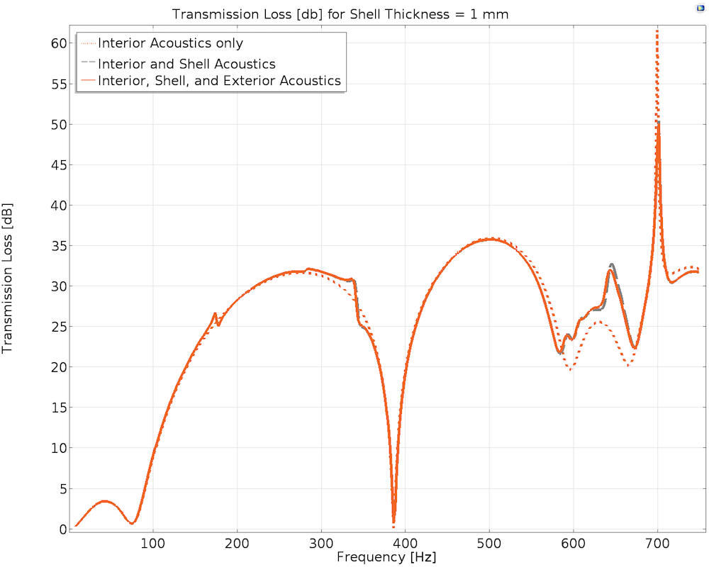
Figure 4. The transmission loss from the muffler inlet to the outlet for a shell thickness of 1 mm.
As expected, the dashed gray curve coincides well with the solid orange curve. The small difference is as expected and derives from air being present on both sides of the shell. The transmission loss is calculated from the muffler inlet to the muffler outlet and the only difference between the two models is the inclusion of the acoustic domain. This indicates that the coupling to the surrounding air domain is essentially one way. The exterior air load on the muffler does not significantly influence the transmission loss. If the outside acoustic domain were stiffer or heavier, its influence on the transmission loss would be more significant. Figure 5 shows the two types of transmission loss computed in this study.
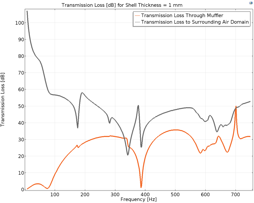
Figure 5. The transmission loss from the muffler inlet to the outlet compared with the transmission loss from the muffler inlet to the acoustic domain boundary.
It is interesting to note that at the lowest computed frequency of 10 Hz, the transmission loss curve for the muffler inlet to the acoustic boundary (solid gray curve) has its peak value of transmission loss. It continues to have a high transmission loss in the low-frequency range below 100 Hz. This implies that in this frequency range, the sound leakage into the surrounding domain is lower in this region than in the rest of the computed frequency range.
However, from the solid orange curve shown in Figure 5, it can be noted that the muffler performance is weak in the range below 100 Hz, with a very low transmission loss relative to the rest of the calculated range. This indicates that the sound is passing through the muffler without much attenuation in the muffler and without exciting the shell of the muffler excessively. This results in a very low sound emission into the surrounding domain.
Sharp dips in the solid gray curve are noted at 172 Hz and 342 Hz, where shell eigenmodes were noted in the previous study. Therefore, more sound is transmitted into the surrounding domain at these frequencies, especially at the mode at 342 Hz (where the solid gray curve shows a lower transmission loss than the solid orange curve). This actually shows that more sound is being emitted into the surrounding acoustic domain than is passing through the muffler outlet.
The third notable dip in the solid gray curve is at 386 Hz, where an acoustic eigenfrequency was found in the previous study. It is interesting to note that at 386 Hz, there is almost no transmission loss from the muffler inlet to the muffler outlet. The orange curve dips close to the y = 0 axis, but the transmission loss in the gray curve at 386 Hz is still above where it is at 342 Hz. This implies that the acoustic mode at 386 Hz is a resonating mode, with the air volume moving back and forth in the muffler cavity without significantly exciting the muffler shell or causing a high sound emission into the surrounding vicinity.
When focusing on two low dips in the solid gray curve (at 172 Hz and 386 Hz) to obtain a better insight into how these two eigenmodes affect the sound radiated from the muffler, isosurface plots of the sound pressure level (SPL) are created for half of the acoustic domain, displayed below in Figure 6.
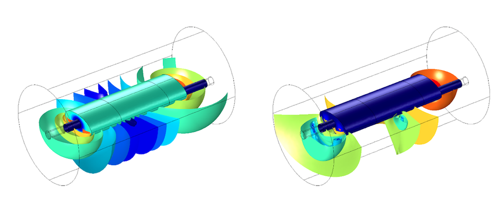
Figure 6. Surface and volume plots for the computed model at 172 Hz (left) and 386 Hz (right).
The figure on the left, for the shell mode at 172 Hz, has the total displacement of the muffler shell plotted along with the isosurfaces of the SPL of the acoustic domain. Maximum shell displacement at 172 Hz occurs at both short ends of the muffler cavity, which creates an almost symmetric distribution of the SPL about the z-axis. On the other hand, the figure on the right has the isosurfaces of the SPL of the acoustic domain accompanying the plot of the SPL of the air contained inside the muffler for the resonating mode at 386 Hz. It is clear that the air contained in the muffler volume is moving back and forth, creating a standing wave. This standing wave inside the muffler volume creates an uneven sound emission into the acoustic domain about the z-axis, due to a higher SPL present at the right end of the muffler.
An eigenfrequency study only goes as far as indicating at what frequency an eigenmode exists. Determining the response of the structure at a specific eigenmode, the behavior of the air in the muffler volume at an eigenfrequency of interest or the interaction of the acoustic and shell modes necessitates a harmonic analysis that consequently yields a transmission loss curve. The transmission loss from the muffler inlet to the muffler outlet obtained in this study and the prior study are able to fulfill this need. Furthermore, the newly defined transmission loss from the muffler inlet to the acoustic domain boundary improves one’s understanding of the muffler’s performance by predicting the sound that is leaked into the surrounding atmosphere.
Thoughts on Predicting the Sound Emission from a Muffler Design
The investigation herein has advanced the investigation from the previous blog post by coupling the muffler model to a surrounding acoustic domain. It has also characterized a new quantity for assessing the performance of the muffler, namely the transmission loss from the muffler inlet to the surrounding atmosphere. The novel technique described here enables muffler designers to better predict external noise generation and therefore meet mandatory noise emission standards.
In an upcoming blog post, this model will be used to evaluate how varying the shell thickness affects the performance of the muffler. Stay tuned!
Note that a shell-stiffening analysis can be conducted in other ways than by simply varying shell thickness. Another method for analyzing the stiffness of the shell could be done by changing the topology of the shell by embossing it and then comparing the embossed shell’s performance to that of the original muffler geometry.
About the Guest Author
Linus Fagerberg from Lightness by Design is an experienced consultant working with simulation-supported product development. He holds a PhD from KTH Royal Institute of Technology and is specialized in the structural mechanics of composites, stability, and optimization. Linus believes that numerical simulation is a great tool to consistently deliver high-quality products, improve performance, and mitigate risks. Lightness by Design is a COMSOL Certified Consultant based in Stockholm, Sweden.


Comments (0)