

While working with rotating components, stability analysis is critical, as instability can lead to catastrophic failure. Rotating systems can lead to unstable responses due to asymmetrical inertia of the disk, asymmetrical stiffness of the shaft, or cross-coupling effects due to bearings. From the designer’s point of view, it’s important to ensure that the potentially unstable modes lie outside the operating range of the machine. Let’s explore how to predict the instability in rotor systems using the COMSOL Multiphysics® software.
What Is Stability?
Stability can be defined as the tendency of a system to move back to its initial equilibrium position. Stability can be classified as:
- Static
- Dynamic
Let’s discuss these two types of stability individually.
Static stability is based on the initial response of a system when disturbed from equilibrium and can be further divided into the following conditions:
- Statically stable: The body tends to return to its equilibrium position after the disturbance
- Statically unstable: The body tends to continue in the direction of the disturbance instead of returning to its equilibrium position
- Neutrally stable: The body remains in equilibrium in the direction of the disturbance after being perturbed
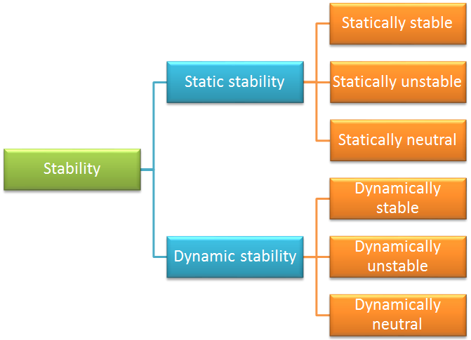
Classification of stability.
Dynamic stability is based on the time history of motion after a system is disturbed from its equilibrium position and can be further divided into the following conditions:
- Dynamically stable: The system’s motion decreases with time
- Dynamically unstable: The system’s motion increases with time
- Dynamically neutral: The system’s motion remains constant with time
These motions are also broadly classified into two categories: oscillatory and nonoscillatory.


Response for oscillatory motion (left) and nonoscillatory motion (right) for different values of the damping coefficient.
As we are now familiar with the basic terminology, let’s get into the mathematical definition of stability and the conditions for which a system becomes unstable.
Defining the Conditions for Stability
The general dynamics equation of motion in inertia is as follows:
where [\textbf M],[\textbf C],[\textbf K] represents the mass, damping, and stiffness matrices, respectively; and \{\textbf u\},\{\textbf F\} represents the displacement and force vectors.
The solution of the dynamic equation can be classified as one of four categories:
- Undamped
- Overdamped
- Underdamped
- Critically damped
The solution for the governing equation is also bounded and well behaved if all of the coefficients are positive. However, there are circumstances in which the coefficients become negative and the solution becomes unbounded. To understand this issue, let’s take a look at the response of a spring-mass-damper system in various scenarios, as shown in the figure below.
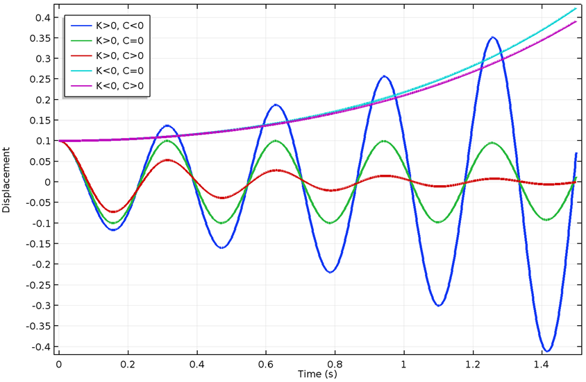
Responses for different values of stiffness and damping coefficients.
From the predicted response of a system, we can say that the system is statically unstable when its stiffness becomes negative and dynamically unstable if the damping becomes negative. We can also point out from the above figure that the system needs to be statically stable in order to be dynamically stable. This is not always the case, especially when gyroscopic effects come into the picture. One common example is a bicycle, which is statically unstable but dynamically stable in a speed range.
Linear stability analysis can be used to predict the instability of a system. The framework of linear stability analysis includes the following steps:
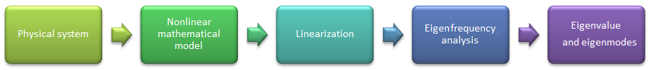
Workflow for a typical linear stability analysis.
Once the eigenvalues are available, the stability can be decided based on the value of the coefficients of the eigenvalue.
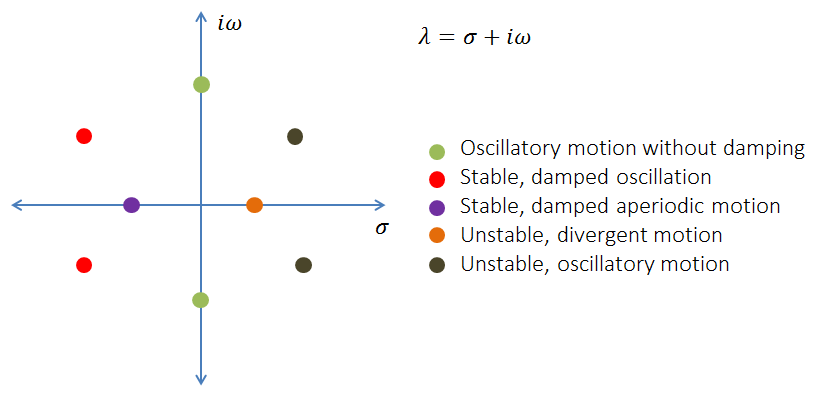
Instead of comparing the coefficients, a better approach is to track the logarithmic decrement, which is defined as \delta= -2\cdot\pi\cdot\frac{\sigma}{\omega}. We can categorize the stability of the system using logarithmic decrement as:
| Value | Type of Behavior |
|---|---|
| \delta < 0 | Unstable |
| \delta > 0 | Stable |
Conditions for instability.
In order to evaluate the logarithmic decrement, you can write it as \delta= -2\cdot\pi\cdot\frac{\Re(\lambda)}{\Im(\lambda)} in terms of eigenvalues. If you are referring to the eigenfrequencies, then it should be written as \delta= 2\cdot\pi\cdot\frac{\Im(\omega)}{\Re(\omega)}.
Equations of Motion for Rotordynamics Problems
Rotordynamics problems are different from conventional vibration analyses. Additional terms appear because of the additional acceleration force terms present in the equation of motion, depending on the selected physics.
In the Rotordynamics Module, there are two approaches to handle the problem. Solid rotors are formulated in a rotating frame and beam rotors are formulated in a stationary frame. The additional terms and effects that appear in the equation of motion, based on the selected physics, are as follows:
| Stationary Frame (Beam Rotor) | Rotating Frame (Solid Rotor) |
|---|---|
| Gyroscopic moments | Coriolis force |
| No centrifugal softening; geometry represented via line | Centrifugal softening |
| No centrifugal stiffening | Centrifugal stiffening |
| Internal damping contribution | External damping contribution |
Now, let’s see how these terms affect the stiffness and damping matrix.
Solid Rotors
The solid rotor is modeled in a rotating frame so that the physical rotation of the rotor is not observed from this frame. The effect of the rotation is accounted for in the momentum balance equation as frame acceleration forces. Because this equation of motion contains extra terms, the equation of motion in rotating frames is:
where \textbf M is the mass matrix; \textbf C_c is the contribution due to the Coriolis effect (depending on the speed of the rotor); \textbf C is the contribution due to external (stationary) and internal (rotating) damping; \textbf K_c is the contribution of external damping in a rotating frame (depending on the speed of the rotor); \textbf K is the stiffness matrix due to internal stiffness, external stiffness, centrifugal softening, and stress stiffening; and \textbf F is the force in the rotating frame.
For solid rotors, you do not get gyroscopic terms; rather, you get centrifugal force (clubbed with the symmetric part of the stiffness matrix), Coriolis force (appears as the antisymmetric part of the damping matrix), Euler force (appears as the antisymmetric stiffness matrix), and the contribution of external damping added as an antisymmetric term in the stiffness matrix.
Beam Rotors
The beam rotor is modeled in a stationary frame. The equation of motion for the rotating frame is:
where \textbf M is the mass matrix; \textbf C_g is the contribution due to the gyroscopic effect (depending on the speed of the rotor); \textbf C is the contribution due to the external (stationary) and internal (rotating) damping; \textbf K_c is the contribution of internal damping in the fixed frame (depending on the speed of the rotor); \textbf K is the stiffness matrix; and \textbf F is the force vector, which contains both the forces and moment (bending and twisting moments on the beam).
In a beam rotor, the gyroscopic terms contribute to the antisymmetric part of the damping matrix and internal damping appears as an antisymmetric term in the stiffness matrix.
How Stiffness and Damping Coefficients Affect Rotor Systems
Consider a shaft whose axis is aligned with the global x-axis. Local y and z directions on the rotor are the same as the global y and z directions.
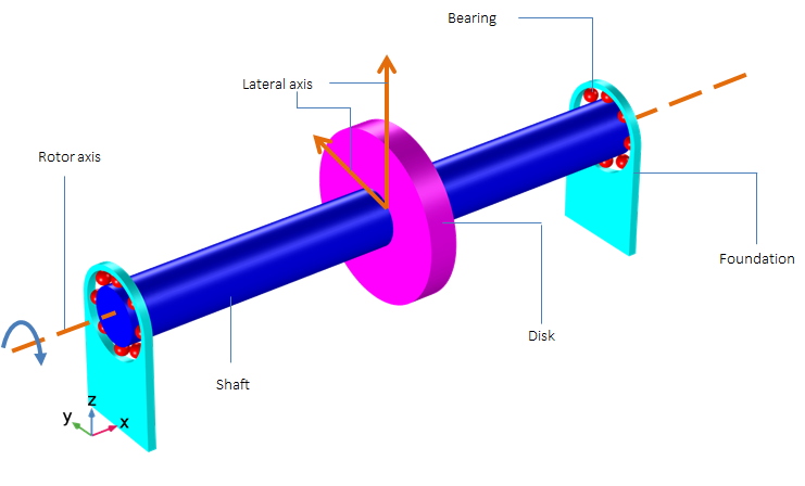
Schematic showing components of a rotor system.
For rotordynamics problems, the lateral equations of motion are coupled; therefore, they are more complex than the equations for axial and torsional vibrations. In this section, we will discuss the effect of direct stiffness and cross-coupled stiffness on the lateral motion of rotors. Let’s consider a symmetric rotor with symmetric bearing on both sides. The bearing contains both direct and cross-coupled terms.
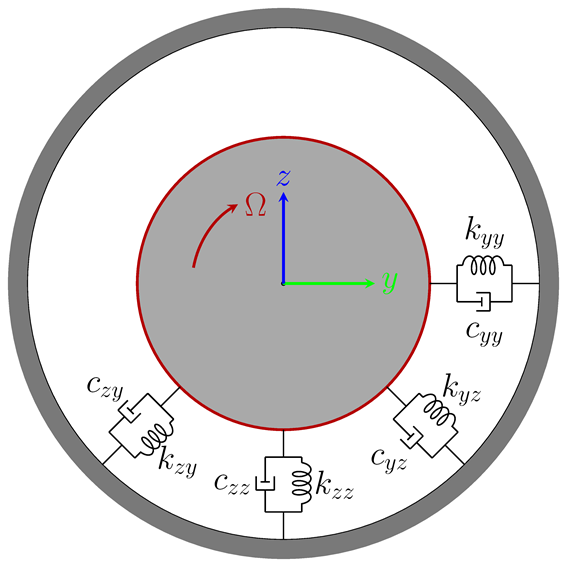
Schematic of a bearing with direct and cross-coupled terms.
If we write the forces in the individual directions, this can be written in matrix form as:
\textbf F_y \\
\textbf F_z
\end{Bmatrix}=-
\begin{bmatrix}
\textbf K_{yy} & \textbf K_{yz}\\
\textbf K_{zy} & \textbf K_{zz}
\end{bmatrix}
\begin{Bmatrix}
\textbf y \\
\textbf z
\end{Bmatrix}-
\begin{bmatrix}
\textbf C_{yy} & \textbf C_{yz}\\
\textbf C_{zy} & \textbf C_{zz}
\end{bmatrix}
\begin{Bmatrix}
\mathbf{\dot{y}} \\
\mathbf{\dot{z}}
\end{Bmatrix}
So, the forces in the y and z directions can be written as:
\textbf F_y = -K_{yy}\cdot\textbf y -K_{yz}\cdot\textbf z -C_{yy}\cdot \dot{\textbf y}- C_{yz}\cdot \dot{\textbf z}\\
\textbf F_z = -K_{zy}\cdot\textbf y -K_{zz}\cdot\textbf z -C_{zy}\cdot \dot{\textbf y}- C_{zz}\cdot \dot{\textbf z}
\end{matrix}
Let’s discuss the individual effect of each term on the lateral motion of the rotor system. Depending on the input, there are two types of whirl modes: forward and backward. In the case of the forward whirl, the orbital motion and the spin direction of the rotor are in same direction, whereas for the backward whirl they are opposite.
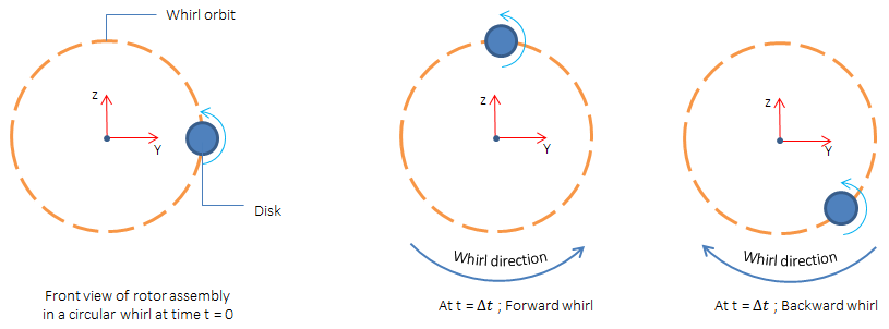
Schematic showing backward and forward whirl.
Direct Coefficients
The direct stiffness terms (\textbf K_{yy}, \textbf K_{zz}) affect forces in the direction of the deflection vector. If the coefficients are positive, then the force is in the opposite direction of deflection. If the coefficient value is negative, then the force is in the same direction as the deflection.
The positive direct damping term (\textbf C_{yy}, \textbf C_{zz}) generates a force normal to the deflection vector and oriented in the direction opposite the whirl velocity. If the values are negative, the forces are oriented in the direction of the whirl velocity.
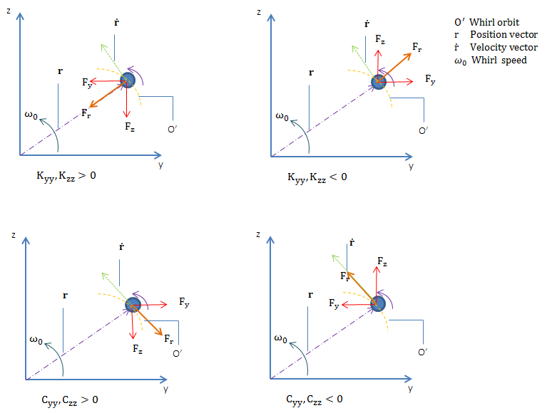
Force diagram for direct stiffness and damping coefficients (forward whirl).
Cross-Coupled Coefficients
If \textbf K_{yz}, \textbf K_{zy} have the same sign, then they produce a force in the direction of the deflection vector or opposite to it based on the sign of the coefficients. If the values of \textbf K_{yz}, \textbf K_{zy} are not the same, then it causes the whirl to become elliptical.
If \textbf K_{yz}, \textbf K_{zy} have opposite signs, then they produce a force normal to the deflection vector. The direction depends on the sign of the coefficient.
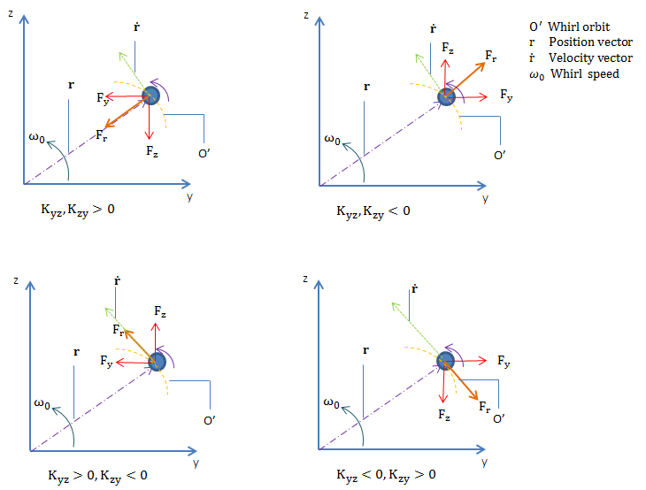
Force diagram for cross-coupled stiffness coefficients (forward whirl).
If \textbf C_{yz}, \textbf C_{zy} have the same sign, then they create a force normal to the deflection vector. The direction depends on the sign of the coefficients. If \textbf C_{yz}, \textbf C_{zy} have different signs, then it creates a force that is collinear with the deflection vector and the sign depends on the coefficients. This produces a stiffening or destiffening effect. For example, if \textbf C_{yz}>0, \textbf C_{zy}<0, then it creates a stiffening effect as the force is directed opposite to the deflection vector.
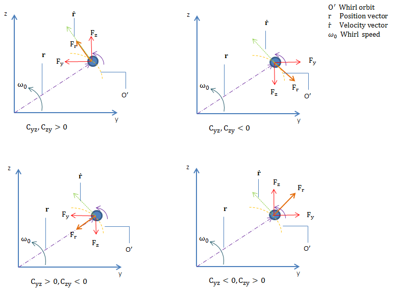
Force diagram for cross-coupled damping coefficients (forward whirl).
In short, the term that generates force in the radial direction (direct stiffness and cross-coupled damping) does not cause instability in the system, while the terms that cause a force tangential to the whirl orbit can cause instability in the system. The effect of the coefficient also varies depending on the whirl modes. For example, if \textbf K_{yz}(+ve), \textbf K_{zy}(-ve), it generates a force tangential to the whirl orbit, which can be destabilizing for the forward whirl and stabilizing for the backward whirl. Let’s summarize the effect based upon the whirl mode:
| Coefficients | Forward Whirl | Backward Whirl | Force Direction |
|---|---|---|---|
| \textbf K_{yy}, \textbf K_{zz} >0 | Stabilizing | Stabilizing | Radial |
| \textbf K_{yy}, \textbf K_{zz} <0 | Destabilizing | Destabilizing | Radial |
| \textbf K_{yz}, \textbf K_{zy} >0 | Stabilizing | Stabilizing | Radial |
| \textbf K_{yz}, \textbf K_{zy} <0 | Stabilizing | Stabilizing | Radial |
| \textbf K_{yz}>0, \textbf K_{zy}<0 | Destabilizing | Stabilizing | Tangential to whirl orbit |
| \textbf K_{yz}0 | Stabilizing | Destabilizing | Tangential to whirl orbit |
| \textbf C_{yz}, \textbf C_{zy} >0 | Destabilizing | Destabilizing | Tangential to whirl orbit |
| \textbf C_{yz}, \textbf C_{zy} <0 | Stabilizing | Stabilizing | Tangential to whirl orbit |
| \textbf C_{yy}, \textbf C_{zz} >0 | Stabilizing | Stabilizing | Tangential to whirl orbit |
| \textbf C_{yy}, \textbf C_{zz} <0 | Destabilizing | Destabilizing | Tangential to whirl orbit |
| \textbf C_{yz}>0, \textbf C_{zy}<0 | Stabilizing | Stabilizing | Radial |
| \textbf C_{yz}0 | Stabilizing | Stabilizing | Radial |
Analyzing Stability in Rotor Systems
As a designer, it is nearly impossible to create a perfect rotor, as there is always some asymmetry present in the model. The asymmetry can be due to mass distribution or in stiffness due to shape. In addition, a rotor can be subjected to cross-coupling forces, internal friction, rotor rubbing, and steam whirl. The presence of these conditions affects the stability of the rotor system. Let’s investigate a few of these cases…
Instability Analysis Due to Bearings
In bearings, the cross-coupling forces are a critical reason for instability. Cross-coupling forces cause rapid loss in the damping of the system and result in subsynchronous rotor vibration. This, in some cases, may lead to zero damping or negative damping, thus making the system unstable.
If the shaft is aligned along the x-axis, then as per common practice, the cross-coupled forces are written in matrix form, as follows:
\textbf F_y\\
\textbf F_z
\end{Bmatrix}=-
\begin{bmatrix}
0 &\textbf K_{yz}) \\
-\textbf K_{yz}& 0
\end{bmatrix}
\begin{Bmatrix}
\textbf y\\
\textbf z
\end{Bmatrix}
Typically, in hydrodynamic bearings, cross-coupled forces play the part of a negative damping in a rotor. When approaching a critical speed, these forces can cause uncontrolled vibration and even failure of the bearing.
A model in the Application Library discusses stability due to cross-coupling forces. The model consists of a turbocharger rotor supported by two bearings: one near the compressor and another near the turbine, making both the compressor and turbine overhung on the shaft.
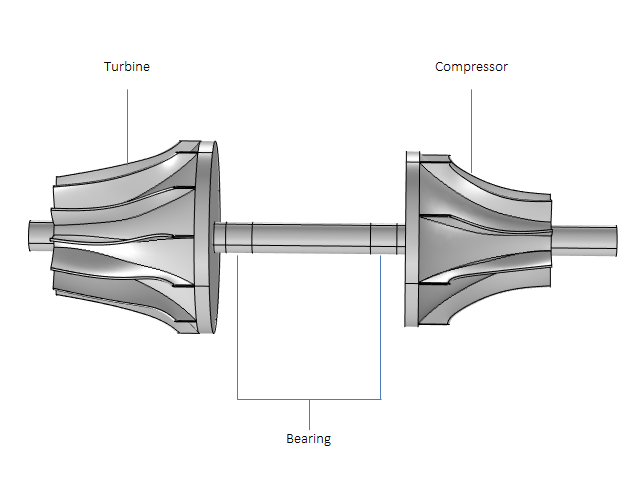
A turbocharger with bearings.
The analysis is run for two cases, one without cross-coupling forces and one with cross-coupling forces. In COMSOL Multiphysics, there are three different ways to include the cross-coupling effects of the bearing:
- If the cross-coupling stiffness is known, it can directly be specified as an off-diagonal stiffness term in the Bearing node
- If the forces are known, they can be specified within the Bearing node using the Forces and Moment option
- To capture the complete nonlinear effects of the bearing, you can directly couple the rotor simulation with the hydrodynamic bearing simulation


Logarithmic decrement without (left) and with (right) a cross-coupled term.
In the plots above, the logarithmic decrement in the absence of cross-coupled stiffness is mostly positive, indicating that the natural modes are stable. Only at high rotational speeds are there a few modes that become unstable. In the presence of cross-coupled stiffness, many modes have a negative logarithmic decrement, even at low rotor speeds.
The results indicate that the presence of cross-coupled stiffness makes the vibrational modes unstable, hence it is dangerous to operate the turbocharger rotor at these speeds.
Instability Due to Rotational Damping
It sounds strange that the element of mechanical dissipation can cause instability, but in the case of a rotating component, it is true. As the rotational damping is attached to the body, it is in the rotating frame. After coordinate transformation in a stationary frame, it is not solely dependent on the velocity anymore. The transformation leads to a dissipative term and a circulatory term, which depend on rotor speed and displacement. The circulatory term is one, which is responsible for the instability.
\mathbf{F_y}\\
\mathbf{F_z}
\end{Bmatrix}=
\begin{bmatrix}
\mathbf{C_i}&\mathbf{0} \\
\mathbf{0}& \mathbf{C_i}
\end{bmatrix}
\begin{Bmatrix}
\mathbf{\dot{y}}\\
\mathbf{\dot{z}}
\end{Bmatrix}
+
\begin{bmatrix}
\mathbf{0}&\mathbf{(C_i\cdot\omega)} \\
\mathbf{-(C_i\cdot\omega)}& 0
\end{bmatrix}
\begin{Bmatrix}
\mathbf{y}\\
\mathbf{z}
\end{Bmatrix}
where \omega is rotor spin speed.
Let’s consider a Laval-Jeffcott rotor that consists of a massless shaft and single disk supported by two identical bearings on ends with symmetric damping and stiffness. Now, if the rotational damping effect is also included in the system, the circulatory term appears in the governing equation and causes instability.
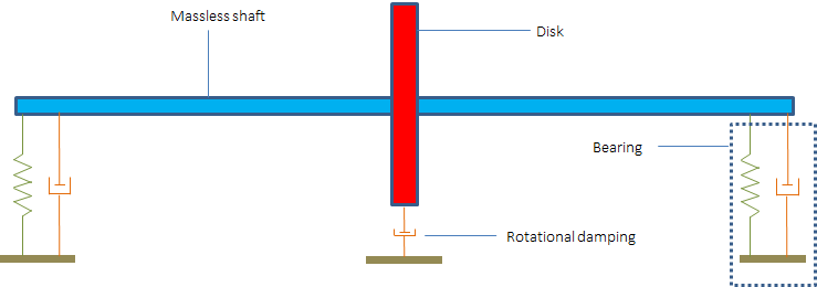
Schematic of a Laval-Jeffcott rotor with internal damping.
To further investigate the effect, let’s draw a force diagram for the system. From the force diagram, it is clear that the circularity term produces force in the direction of motion for forward whirl. This means that the circulatory term is adding energy to the system, while the dissipative term due to external damping continuously removes the energy from the system.
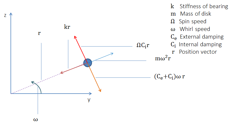
Force diagram for a Laval-Jeffcott rotor with internal damping.
From the force diagram, we can say that the condition \Omega = \omega \frac{C_e+C_i}{C_i} triggers instability in cases of asynchronous whirl conditions. Asynchronous whirl occurs when the spin speed and whirl frequency are not the same. The internal damping in rotors is produced by either the material’s hysteretic damping or by the Coulomb damping due to rubbing at the interface of shrink-fitted parts.
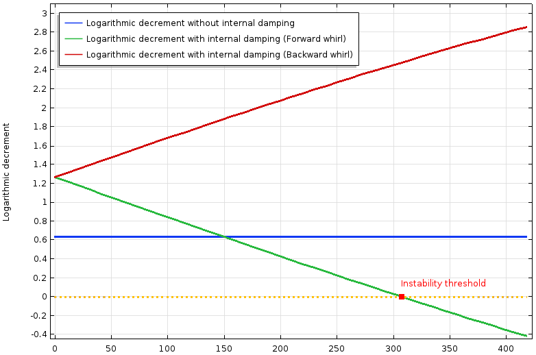
Logarithmic decrement of a Laval-Jeffcott rotor without internal damping (blue) and with internal damping (red and green).
The plot above compares a rotor model with and without internal damping. The forces due to the cross-coupling term are nonconservative in nature. The internal damping contributes to the stiffness matrix as a cross-coupling term, which depends on the speed, so the logarithmic decrement is not constant and varies with the speed. The logarithmic decrement is plotted for two initial modes, the forward and backward modes. At zero spin, both the modes have the same logarithmic decrement. As the speed increases, the logarithmic decrement increases for the backward whirl, decreases for the forward whirl, and finally becomes negative. This confirms that the cross-coupling term stabilizes the backward whirl and destabilizes the forward whirl.
If we perform a frequency-domain analysis, the results are identical to the case without damping and the whirl is circular. This means that there is only forward whirl in the model.
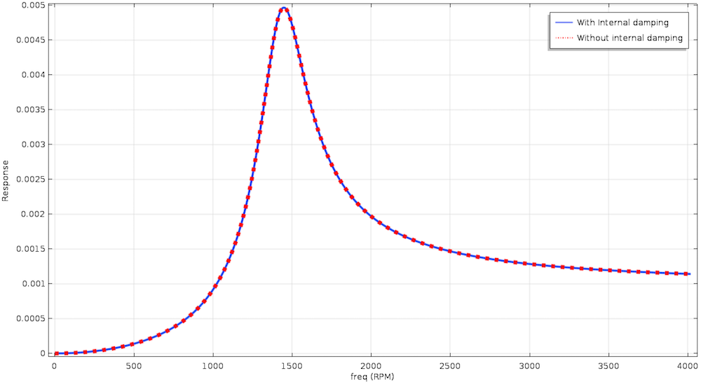
Frequency response of a Laval-Jeffcott rotor with and without internal damping.
A cross-coupling term due to rotational damping only affects the damping characteristics without changing the response of the system. Now, if we look at the Campbell diagram, the natural frequency is no longer a constant value, or else it increases with the speed if internal damping is present. The effect increases the damped critical speed in cases of internal damping or if we want to find the instability threshold using the Campbell diagram. Then, we can draw a line \omega=\Omega(\frac{C_i}{C_i+C_e})\ and the intersection of the line with the natural frequency gives the threshold value.
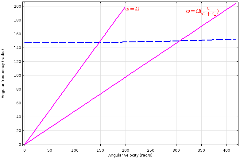
Campbell diagram of a Laval-Jeffcott rotor with internal damping for initial mode.
Instability Due to Steam Whirl
Steam whirl arises in axial flow machines, like gas turbines, when the radial displacement of the shaft takes place as a result of leakage along the circumference. This sets up a resultant force perpendicular to the displacement. The excited force gives instability for some operating conditions and stability for others. The steam whirl force adds to the stiffness term in a skew-symmetric way, like internal damping, but there is no dependency on the spin speed.
\mathbf{F_y}\\
\mathbf{F_z}
\end{Bmatrix}=
\begin{bmatrix}
\mathbf{0}&\mathbf{(K_{sw})} \\
-\mathbf{(K_{sw})}& 0
\end{bmatrix}
\begin{Bmatrix}
\mathbf{y}\\
\mathbf{z}
\end{Bmatrix}
To understand the effect more easily, let’s discuss the force diagram for a Laval-Jeffcott rotor with external damping and stiffness subjected to steam whirl.
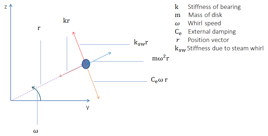
Force diagram for a Laval-Jeffcott rotor with steam whirl.
From the force diagram, we can see what the stability threshold is when K_{sw}=C_e\cdot\omega_n, where \text{\math{\omega_n}$} is the natural frequency. This means that the stability threshold can be increased by increasing the external damping or natural frequency.
Let’s consider a Laval-Jeffcott rotor such that the system is initially unstable due to the skew-symmetric term. If we introduce external damping into the system, the logarithmic decrement moves toward zero and finally becomes positive. By increasing the value of the external damping, the frequency value of the system’s instability threshold can be increased.
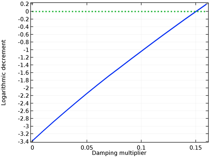
Logarithmic decrement of a Laval-Jeffcott rotor with fixed ends and steam whirl.
Concluding Thoughts
In this blog post, we discuss the types of stability, influence of the coefficients of damping and stiffness matrices over the response of the system, governing equations for solid rotor and beam rotor physics, methods to predict the instability in a system using eigenfrequency analysis, and a few applications that induce instability in rotor systems.
Next Steps
Learn more about the specialized features for modeling rotating systems available in the Rotordynamics Module, an add-on to COMSOL Multiphysics and the Structural Mechanics Module, by clicking the button below.

Comments (1)
Harsh Goel
October 27, 2020Hello
I read the blog and is very informative. I had a model wherein I want to combine solid rotor and beam rotor. Is it possible to do so?
Thanks in advance.