
In this first blog entry of our new solver series, we describe the algorithm used to solve all linear static finite element problems. This information is presented in the context of a very simple 1D finite element problem, but is applicable for all cases, and is important for understanding more complex nonlinear and multiphysics solution techniques to be discussed in upcoming blog posts.
What Makes a Finite Element Model Linear and Static
Consider the system shown below, of a spring that is attached to a rigid wall at one end, and with an applied force at the other end.
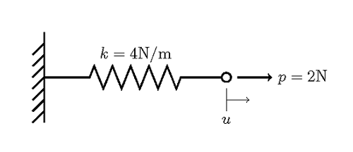
We are interested in finding the displacement of the end of the spring, where the force is applied. Using the vocabulary of the finite element method, we have here a single element finite element model. The spring is the element, and it is bounded by two nodes at either end. One of the nodes is fixed rigidly to the wall, and other node will deform due to the applied load. We are trying to find the nodal displacements due to the applied load. This problem is linear because neither the material properties (the spring constant) nor the loads are dependent upon the solution. This is a static problem because we are finding the solution under the assumption that there is no variation with respect to time.
Working Through the Model
This problem can easily be solved with pen and paper, but let’s look at how this is done in a more rigorous way. Consider the node where we are trying to find the displacement, and draw the balance of forces at equilibrium:
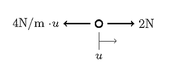
We can write this out as: f(u)=p-ku, and we call this equation the functional of the system, at equilibrium (steady state conditions) the functional is equal to zero. We want to find the value of u such that f(u)=0. Let’s also plot out the functional:
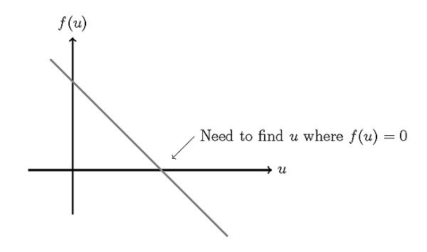
Of course we can find the solution by examination in this case, but in general u will be a vector with possibly millions of unknowns, so let’s be more rigorous and take a look at the exact algorithm used:
- Choose a starting guess, for example: u_{init}=0
- Evaluate the functional at this point: f(u_{init})=2-4(0)=2
- Evaluate the derivative of the functional: f'(u_{init})=-4
- Compute the solution: u_{solution}=u_{init}-[f'(u_{init})]^{-1}f(u_{init})=0-(2/(-4))=0.5
The above algorithm is also known as the Newton-Raphson method. Additionally, we can visualize this graphically as:
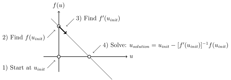
Note that regardless of the starting point, the solution will be found in one step. So, whenever you solve a linear static finite element problem in COMSOL Multiphysics, the software is following this algorithm to find the solution. Now, the above example has only a single unknown, so we only need to solve a single linear equation. Typically your models will have thousands or even millions of unknowns, which means you will need to solve a system of linear equations, but the idea is the same.
Lastly, we address the issue of numerical scaling. Whenever we solve a problem on a computer, we need to consider the problem of finite precision due to the floating point representation of numbers. Computers cannot represent the space of the real numbers perfectly. To minimize the effect of this, COMSOL applies a scale factor to the equations before they are solved. COMSOL automatically chooses a scaling appropriate for each set-up field variables in the model, and this almost never needs to be handled by the user, but it is worth knowing what effect the scale factor has. As long as it is within a few orders of magnitude of the average magnitude of the values in the solution, then no interaction is required. Only if the scaling is very different from the expected solution magnitude should the scale factor be changed.
To summarize what you need to know about solving linear static finite element models:
- Regardless of what starting guess you use, you will find the solution in one iteration
- The scaling of the variables is done to address the issue of finite precision floating point arithmetic
How to Interpret the COMSOL Log File
The Log File
Now let’s look at how the above information can be used to interpret the COMSOL Log file of a typical linear static finite element model. Here’s the log file (with line numbers added) from a thermal stress problem:
1) Stationary Solver 1 in Solver 1 started at 30-Apr-2013 17:41:45.
2) Linear solver
3) Number of degrees of freedom solved for: 3651 (plus 124 internal DOFs).
4) Symmetric matrices found.
5) Scales for dependent variables:
6) Displacement field (Material) (mod1.u): 0.0090
7) Temperature (mod1.T): 2.9e+002
8) Iter     Damping    Stepsize #Res #Jac #Sol
9)   1   1.0000000    4.7e-017    1    1    1
10) Stationary Solver 1 in Solver 1: Solution time: 0 s
11)                                 Physical memory: 878 MB
12)                                 Virtual memory: 879 MB
Explanations
- Line 1 reports the type of solver called, and the start time.
- Line 2 reports that the software is calling the linear system solver. (COMSOL can automatically detect if the problem is linear or nonlinear, and will call the appropriate solver.)
- Line 3 reports the size of the problem in terms of the number of degrees of freedom (DOF). The internal DOF’s (when they are used at all) typically are used to compute boundary fluxes, and do not significantly affect problem size.
- Line 4 reports on the type of finite element matrix to be solved.
- Lines 5-7 report the scaling. In this case, a thermal stress problem is solved, so COMSOL scales the displacement and temperature fields. The displacement field scale is 0.0090, using the unit system of the model (meters) so as long as the structural displacements are not smaller than ~9 nanometers (or larger than 9 km!) this scaling is acceptable for displacement. The temperature field scale factor is 293 K. Unless we’re solving a cryogenic problem (where the temperatures may be 4 K +/- 0.001 K) or a problem with temperatures in the millions of Kelvin, this scaling is also acceptable.
- Lines 8-9 report that a single Newton-Raphson iteration was used to solve this problem.
- Lines 10-12 report the solution time and memory requirements.
Now you should have an understanding of how linear static problems are solved in COMSOL, and how to interpret the log file.



Comments (7)
John Pinckney
October 16, 2013Thanks Walter, looking forward to you next posts.
Ivar Kjelberg
October 18, 2013Hi Walter
What about bouncing off this blog post, and use it as an example to illustrate how to decide for appropriate local meshing density?
=> to allow to locally resolve the dependent variable gradients.
One of the strong points of COMSOL is to mesh once the physics has been defined, which allows so nicely to couple all these “physics” together, hence putting back the meshing operation where it belongs: a final “mathematical” discretization of the domains (with obvious similarity to sound sampling theory).
At the point u_init = 0, you say above that one need to estimate the derivative f'(u_init).
From my knowledge this is done (when the full set of equations cannot be analytically derived) by taking difference between mesh nodes, hence you should at least have one mesh node between u_init and your u_solution (even if u_solution is unknown).
For many physics the value of f ‘(u_init) can be estimated:
i.e. in thermal diffusion, for temporal models, the known thermal diffusivity alpha_T [m^2/s] = k/rho/Cp gives a good link between the mesh spatial extend Dz and the related minimum time stepping by respecting Dt > N*Dz^2/alpha_T. Using a N=2 gives a reasonable mesh size to just pass the Nyquist criteria such to evaluate grad(T), hence to avoid negative absolute temperatures (or negative concentration for chemical diffusion) when solving.
I hope you have more time than me to put this together in a clearer and better illustrated way, here on the COMSOL blog
And thanks again for your series of well written texts
Sincerely
Ivar
Birru Mahendar
October 21, 2013Conceptual. Easy to understand Comsol working. Thanks Walter.
Walter Frei
October 22, 2013Thanks Ivar, you may want to see my latest post on meshing (http://www.comsol.com/blogs/meshing-considerations-linear-static-problems/). I’m planning a few more following that as well.
xu yang
November 26, 2015HI Walter, what is the actual mean of Damping Stepsize #Res #Jac #Sol?
Iter Damping Stepsize #Res #Jac #Sol
9) 1 1.0000000 4.7e-017 1 1 1
Walter Frei
November 30, 2015Hello Xu, For detailed information about all of these quantities, please also consult the documentation.
Evgeni Sergeev
March 4, 2016An easy way to tell if the problem is linear, is to ask: if we scale all the BCs and source terms by the same factor F, is the solution now going to be the same as before, scaled by F? If so, then it’s a linear problem.