COMSOL Multiphysics^® 6.0 Release Highlights

Corrosion Module Updates

For users of the Corrosion Module, COMSOL Multiphysics^® version 6.0 brings a new Cathodic Protection interface, a new predefined formulation for adsorption-desorption in combination with electrode reactions, and several new tutorial models. Learn more about these updates below.

New Cathodic Protection Interface

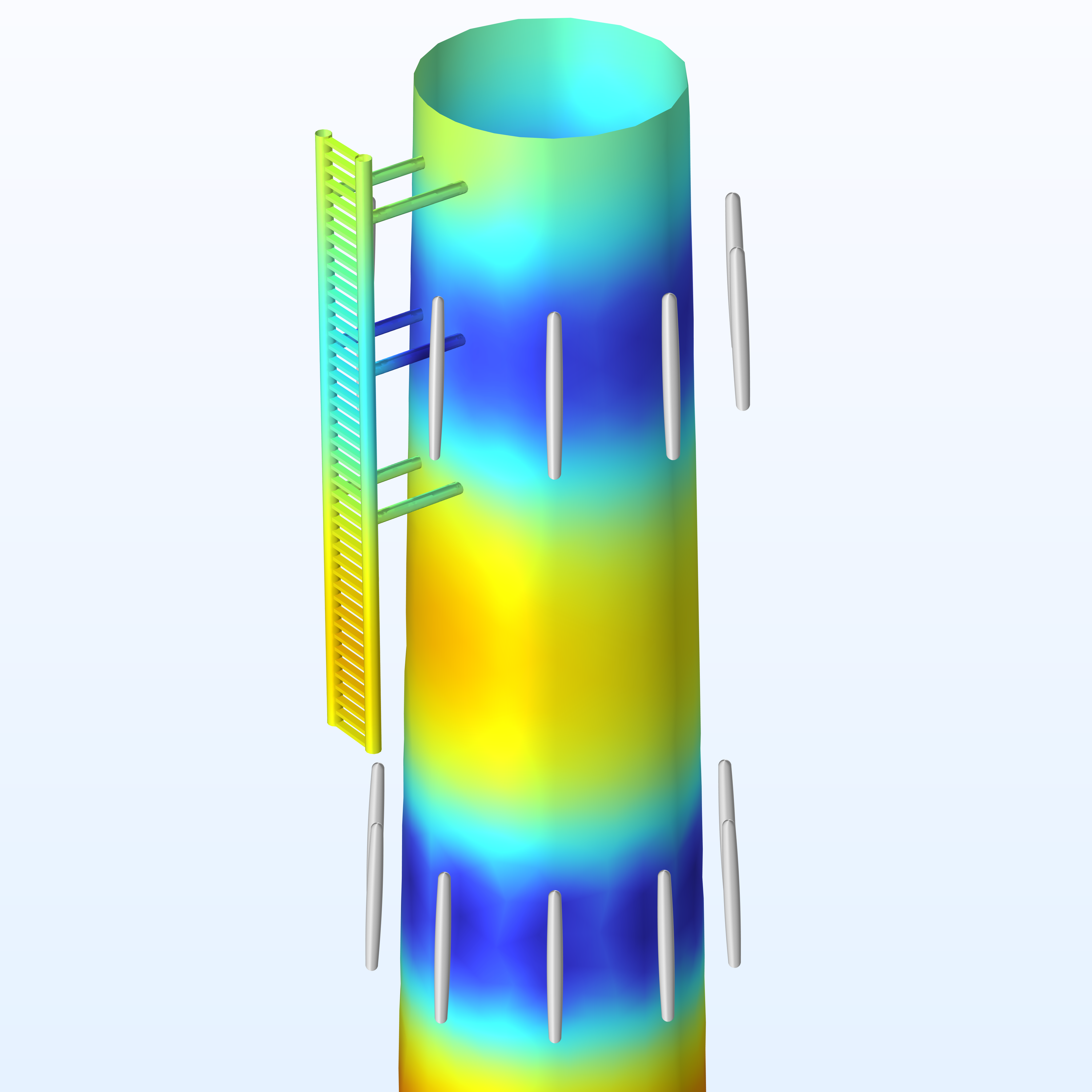
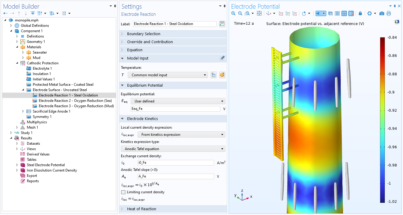
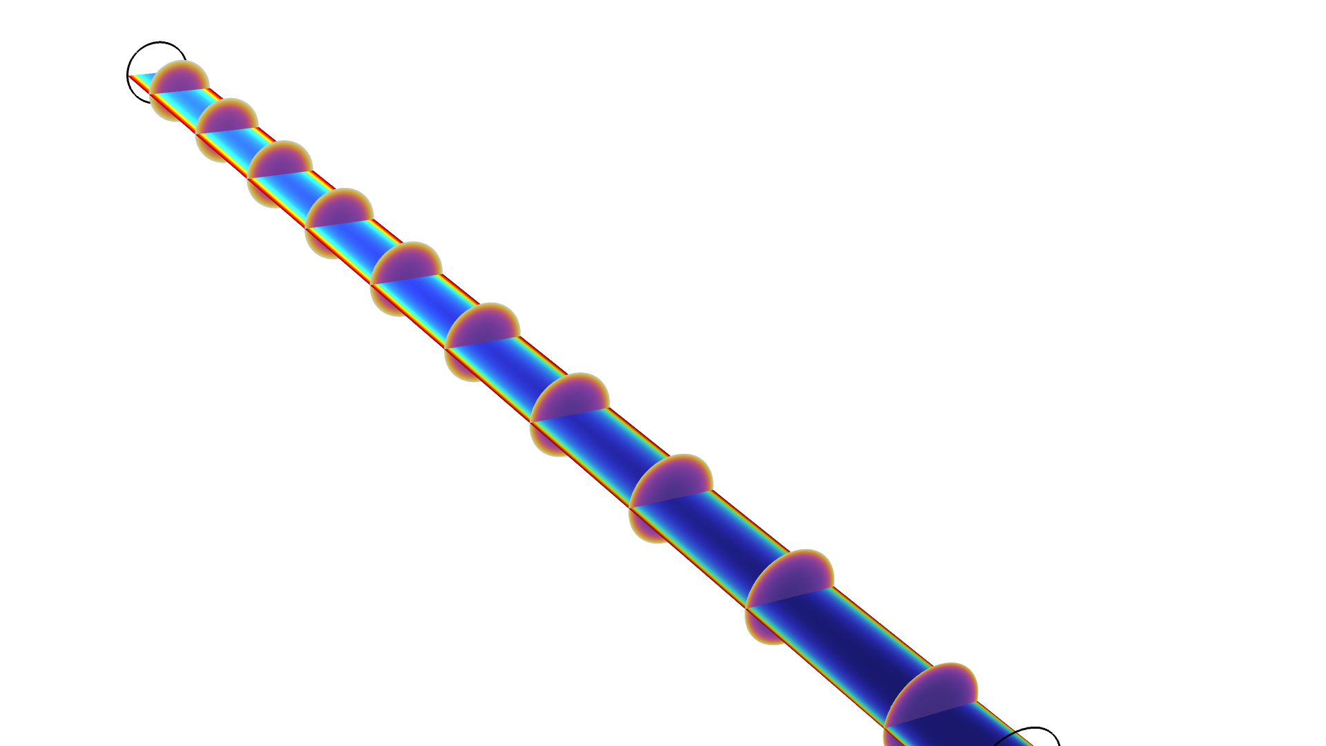
A new Cathodic Protection interface, based on secondary current distribution, allows you to define impressed current, connection, passive metal, protected metal, and thin passive metal surfaces. Settings such as control potential, protected surface sense potential, and reference electrode potentials edit fields are available for easier problem definition. The limiting current for oxygen reduction at protected surfaces can also be entered. You can view this new interface in the following tutorial models:

• monopile_with_dissolving_sacrificial_anodes
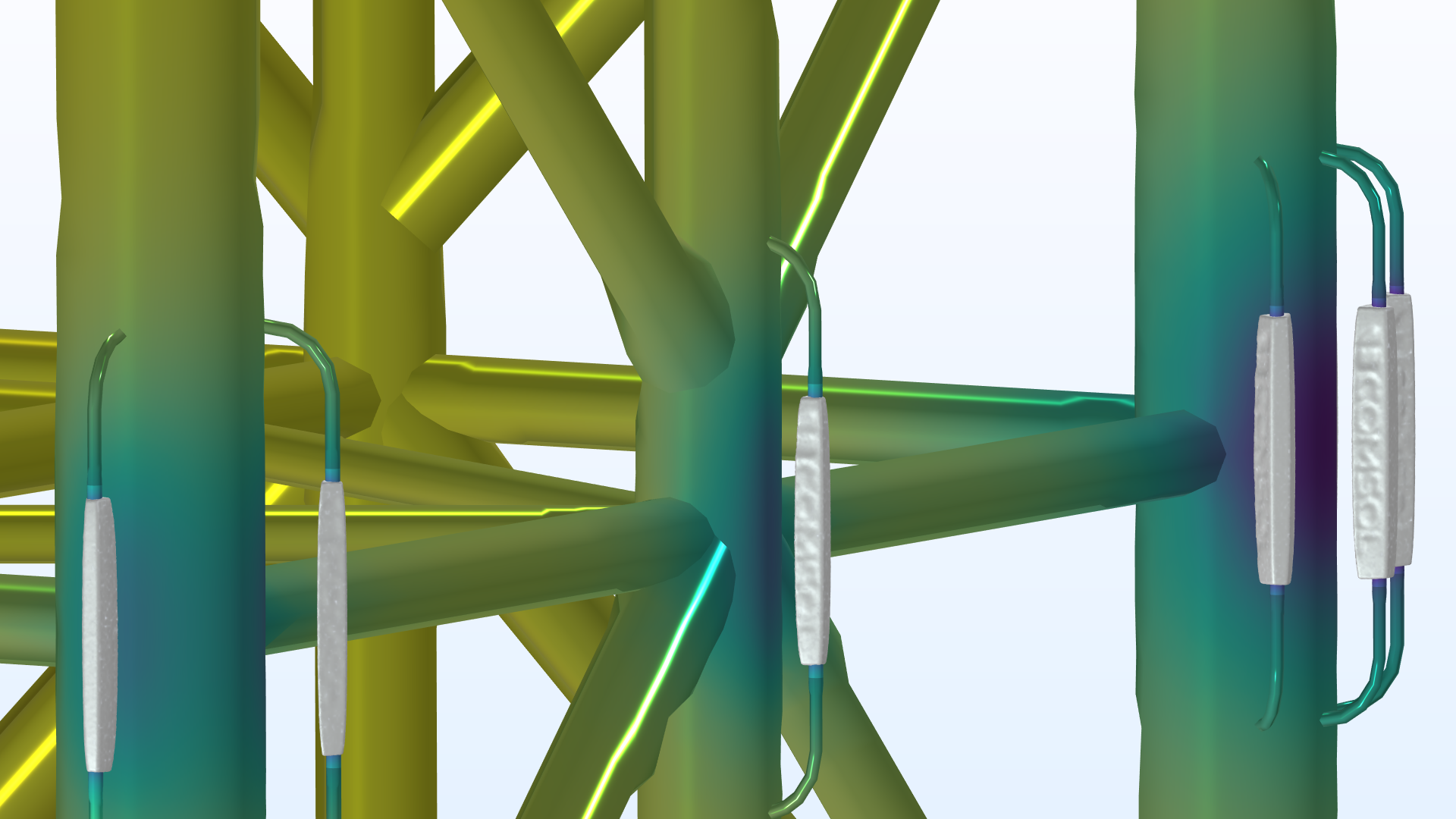
• corrosion_protection_of_an_oil_platform_using_sacrificial_anodes
• corrosion_protection_of_a_ship_hull

The electrode surface potential of the upper part of a monopile.

Adsorbing-Desorbing Species

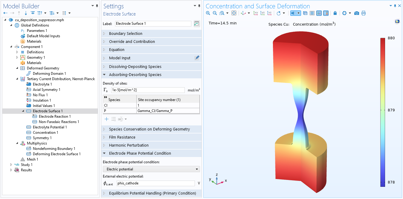
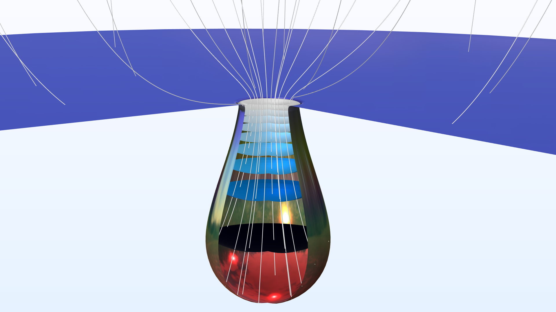
The modeling capabilities of the existing Electrode Surface boundary condition have been expanded with a set of predefined equations that keep track of surface site occupancy and surface concentration of adsorbed species. The new Adsorbing-Desorbing Species section allows you to model the adsorption-desorption kinetics and thermodynamics at electrode surfaces in combination with multistep electrochemical reactions. You can see this feature in the Copper Deposition in a Through-Hole Via, Adsorption-Desorption Voltammetry tutorial model.

The concentration variation in a deformed geometry of a through-hole via after copper deposition.

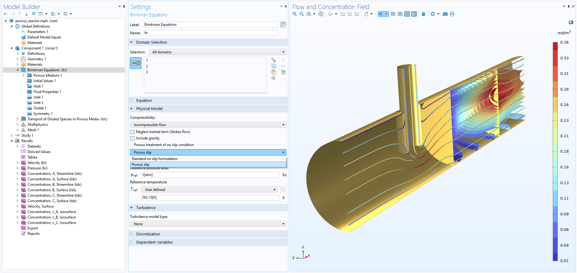
Porous Slip for the Brinkman Equations Interface

The boundary layer in flow in porous media may be very thin and impractical to resolve in a Brinkman equations model. The new Porous slip wall treatment feature allows you to account for walls without resolving the full flow profile in the boundary layer. Instead, a stress condition is applied at the surfaces, yielding decent accuracy in bulk flow by utilizing an asymptotic solution of the boundary layer velocity profile. The functionality is activated in the Brinkman Equations interface Settings window and is then used for the default wall condition. You can use this new feature in most problems involving subsurface flow described by the Brinkman equations and where the model domain is large.

The flow and concentration field of a porous reactor model.

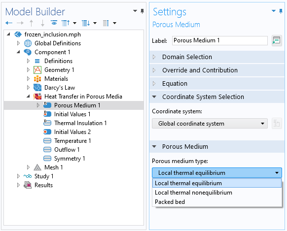
Heat Transfer in Porous Media

The heat transfer in porous media functionality has been revamped to make it more user friendly. A new Porous Media physics area is now available under the Heat Transfer branch and includes the Heat Transfer in Porous Media, Local Thermal Nonequilibrium, and Heat Transfer in Packed Bed interfaces. All of these interfaces are similar in function, the difference being that the default Porous Medium node within all these interfaces has one of three options selected: Local thermal equilibrium, Local thermal nonequilibrium, or Packed bed. The latter option has been described above and the Local Thermal Nonequilibrium interface has replaced the multiphysics coupling and corresponds to a two-temperature model, one for the fluid phase and one for the solid phase. Typical applications can involve rapid heating or cooling of a porous medium due to strong convection in the liquid phase and high conduction in the solid phase like in metal foams. When the Local Thermal Equilibrium interface is selected, new averaging options are available to define the effective thermal conductivity depending on the porous medium configuration.

In addition, postprocessing variables are available in a unified way for homogenized quantities for the three types of porous media. View the new porous media additions in these existing tutorial models:

• freeze_drying
• frozen_inclusion
• porous_microchannel_heat_sink_optimization
• geothermal_doublet

Nonisothermal Flow in Porous Media

The new Nonisothermal Flow, Brinkman Equations multiphysics interface automatically adds the coupling between heat transfer and fluid flow in porous media. It combines the Heat Transfer in Porous Media and Brinkman Equations interfaces.

The tutorial example Free Convection in a Porous Medium makes use of the new nonisothermal flow functionality. Temperature (K) in a porous structure subjected to temperature gradients and subsequent free convection.

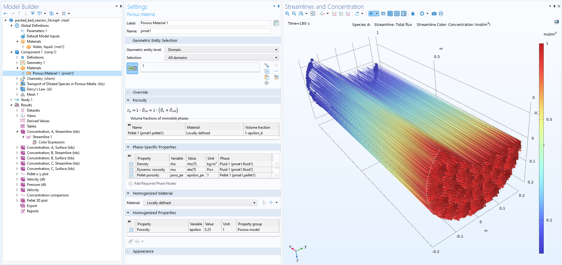
Greatly Improved Handling of Porous Materials

Porous materials are now defined in the Phase-Specific Properties table in the Porous Material node. In addition, subnodes may be added for the solid and fluid features where several subnodes may be defined for each phase. This allows for the use of one and the same porous material for fluid flow, chemical species transport, and heat transfer without having to duplicate material properties and settings.

Nonisothermal Reacting Flow

There are now Nonisothermal Reacting Flow multiphysics interfaces that automatically set up nonisothermal reacting flow models. The Reacting Flow multiphysics coupling now includes the option to couple the Chemistry and Heat Transfer interfaces. Using this coupling, the cross-contributions between heat and species equations like enthalpy of phase change or the enthalpy diffusion term are included in the model. The temperature, pressure, and concentration dependence of different quantities and material properties are also automatically accounted for, making it possible to perform heat and energy balance using the corresponding predefined variables. View this new feature in the existing Dissociation in a Tubular Reactor tutorial model.

Temperature distribution in a tubular reactor.

New and Updated Tutorial Models

COMSOL Multiphysics^® version 6.0 brings several new and updated tutorial models to the Corrosion Module.

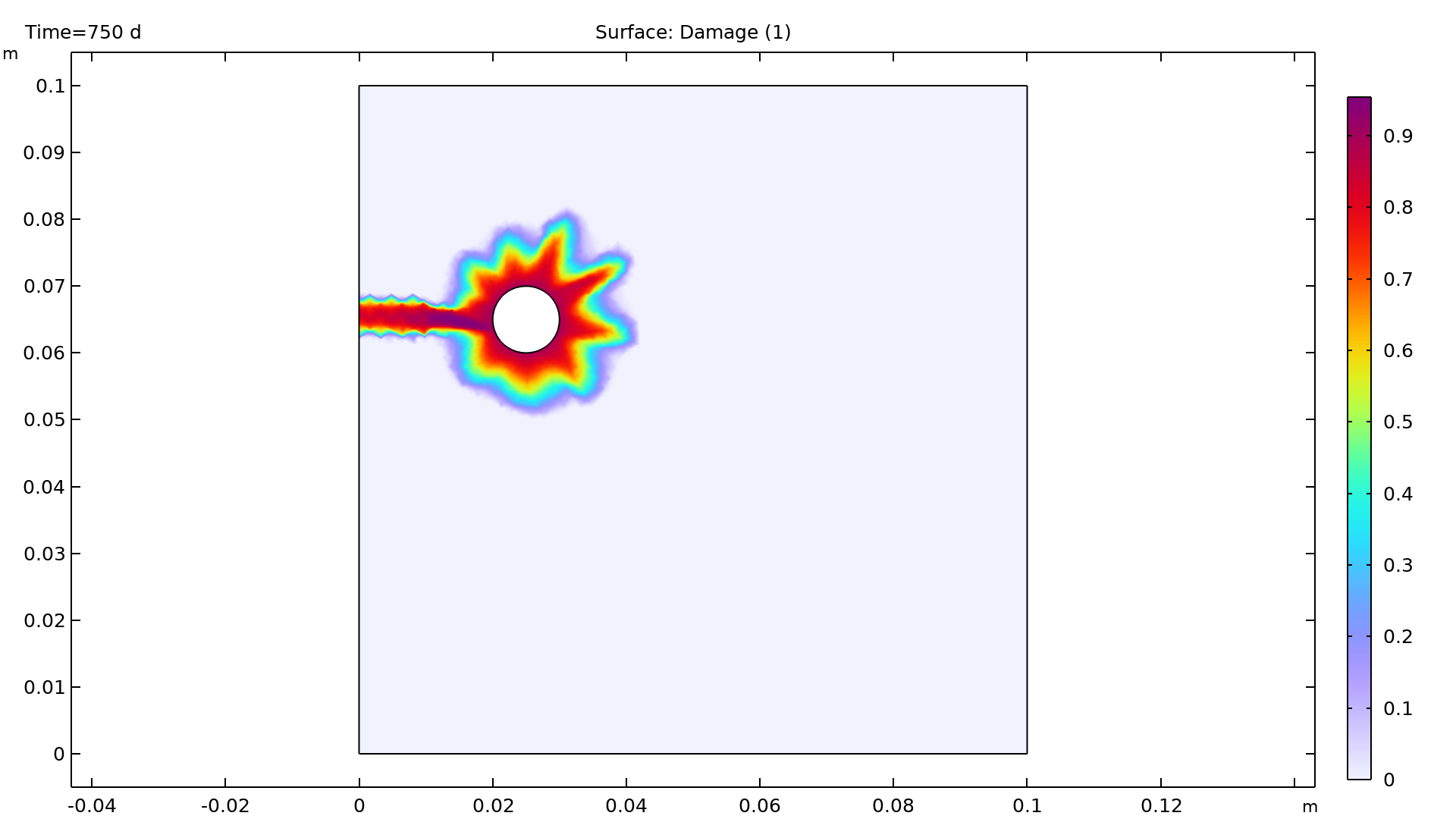
Pitting Corrosion

This tutorial investigates the fundamental mechanism of pit propagation in pitting corrosion by modeling electrode kinetics, mass transport, charge transport, and the resulting geometry deformation of the metal as the pit grows.

Application Library Title:
pitting_corrosion
Download from the Application Gallery

Cathodic Protection with Deforming Anodes

Cathodic protection of an oil rig structure. The sacrificial anodes (gray) are consumed over time. The shape change during this process is modeled by coupling the Cathodic Protection interface with the Level Set interface.

Application Library Title:
cp_with_anode_deformation
Download from the Application Gallery

Oxide Jacking of Reinforced Concrete

This example models oxide jacking of reinforced concrete. The corrosion process causes growth of an oxide layer on the rebar, which in turn causes internal stresses in the concrete.

Application Library Title:
oxide_jacking
Download from the Application Gallery