Ray Optics Module Updates
For users of the Ray Optics Module, COMSOL Multiphysics® version 6.0 features a significantly improved and updated Optical material library in which structural and thermal properties are listed alongside optical dispersion coefficients and internal transmittance data for more than 500 optical glasses. Elsewhere, new ray release features have been introduced for modeling Gaussian beams and the emission of blackbody radiation from surfaces.
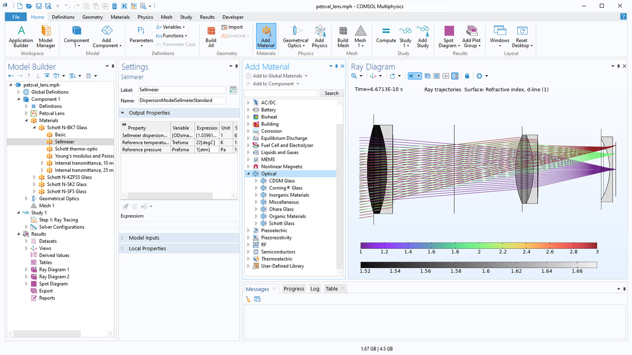
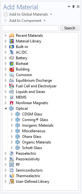
Optical Material Library Improvements
In the Optical material library, available for the Ray Optics Module and Wave Optics Module, glasses from SCHOTT AG, CDGM Glass Company Ltd., Ohara Corporation, and Corning Inc. are now presented with more comprehensive material data. In addition to optical dispersion coefficients and thermo-optic coefficients, many of these glasses now include internal transmittance, density, Young's modulus, Poisson's ratio, coefficient of linear thermal expansion, thermal conductivity, and specific heat capacity. With the inclusion of more comprehensive material data for optical glasses, it is now easier than ever to set up coupled structural-thermal-optical performance (STOP) analysis models.
You can see these improvements in the new Petzval Lens Optimization model and these existing tutorial models:
- cross_grating_echelle_spectrograph
- double_gauss_lens
- double_gauss_lens_image_simulation
- gregory_maksutov_telescope
- light_pipe
- petzval_lens_geometric_modulation_transfer_function
- petzval_lens_stop_analysis
- petzval_lens_stop_analysis_isothermal_sweep
- petzval_lens_stop_analysis_with_hyperelasticity
- petzval_lens_stop_analysis_with_surface_to_surface_radiation
- petzval_lens
- schmidt_cassegrain_telescope
- white_pupil_echelle_spectrograph
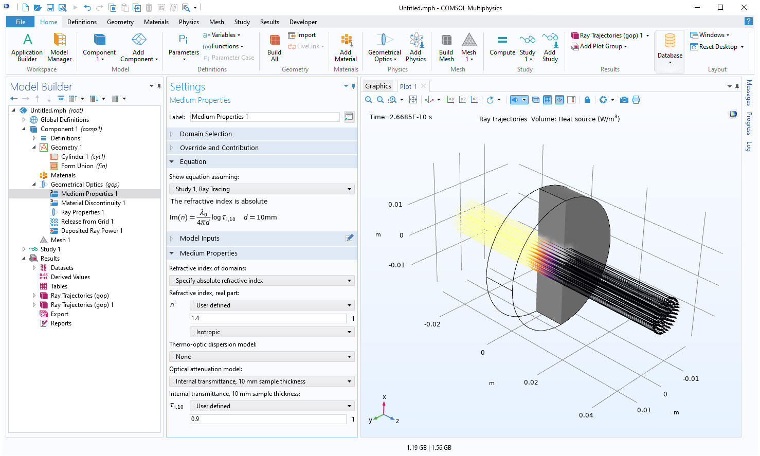
New Ways to Define Absorbing Media
In the Geometrical Optics interface, there are new ways to define an absorbing medium. For one, you can simply specify the attenuation coefficient. Alternatively, you can enter the internal transmittance, which is the fraction of light intensity that would be transmitted through a material sample of a given thickness while neglecting Fresnel losses at the surfaces. Many of the materials in the Optical material library now control the absorption characteristics by including lookup tables of internal transmittance data. In previous versions, the only way to set up an absorbing medium was by entering the real and imaginary parts of the refractive index directly (the imaginary part or negative imaginary part is sometimes called the extinction coefficient).
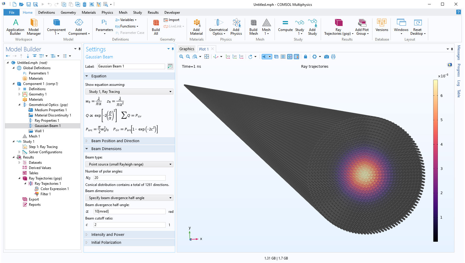
Gaussian Beam Ray Release Feature
The Gaussian Beam ray release feature is now available when solving for the ray intensity or power. It can be added to release rays with a Gaussian distribution of initial intensity or power. You can specify the beam waist radius, beam divergence half-angle, or Rayleigh range; the intensity profile of the beam is then computed automatically. The Gaussian Beam feature can be used in two different ways. If the Rayleigh range of the beam is very small compared to the model geometry, then this feature treats the beam as a point source, from which the rays follow a conical distribution with angle-dependent initial intensity. Alternatively, if the Rayleigh range is significantly larger than the geometry size, you can release a collimated beam in which the rays all follow parallel paths.
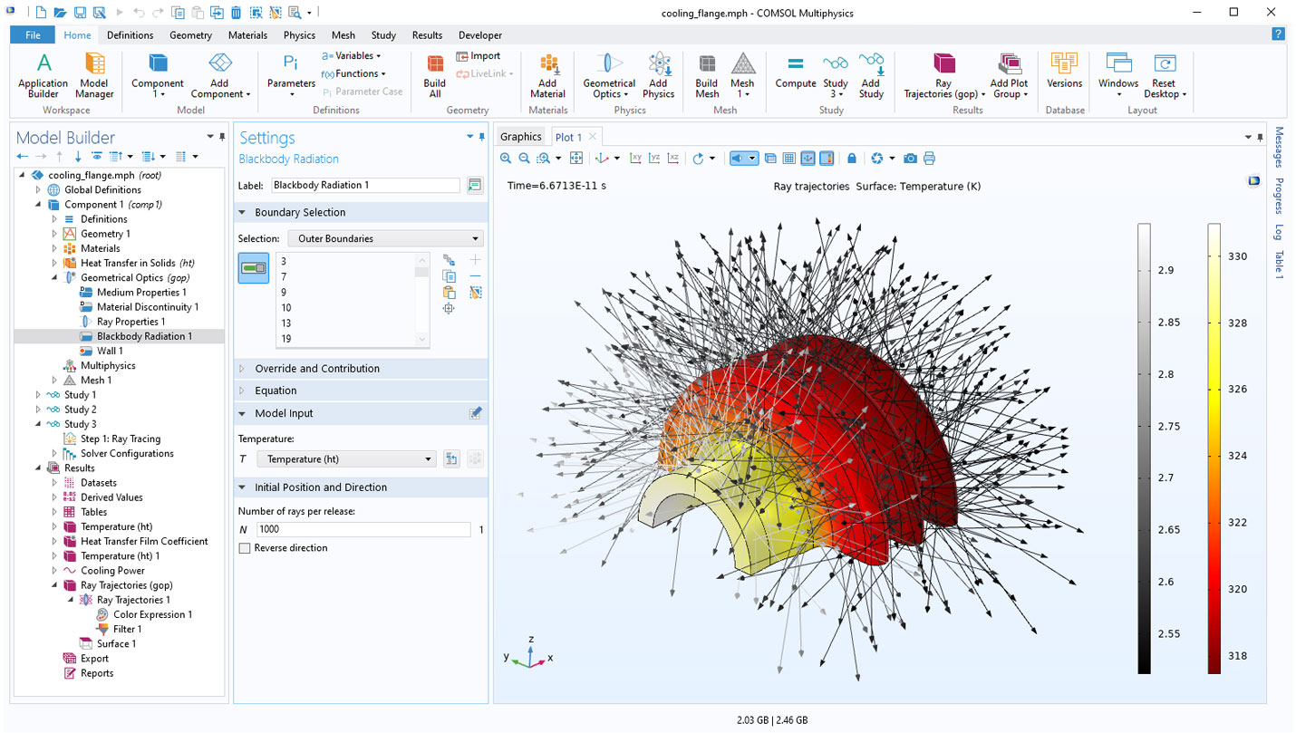
Blackbody Radiation Ray Release Feature
You can now release rays from a surface with the power and wavelength distribution of an ideal blackbody radiation source. The dedicated Blackbody Radiation feature, available in 3D models, assigns the initial intensity and power of released rays based on the surface temperature. If the Geometrical Optics interface has been configured to allow release of polychromatic light, then the wavelength or frequency of rays is automatically sampled from a Planck distribution function based on the surface temperature. The more general ray release features, such as Release from Grid and Release from Boundary, also allow you to release polychromatic light following a Planck distribution, although in this case the initial ray intensity and power are specified separately.
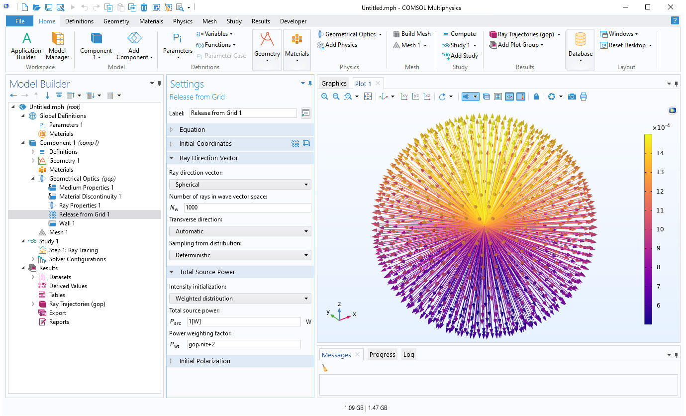
New Ways to Specify Initial Intensity Distribution
New settings are available to release rays with a weighted distribution of initial ray power. In the settings for most ray release features, such as Release or Release from Grid, you can choose to assign a Weighted distribution of initial intensity or power. The total power over all rays will still add up to the specified total source power, but the power of individual rays can be proportional to a weighting factor, which could be a function of initial ray position and direction. This could be used to assign directivity to custom ray sources.
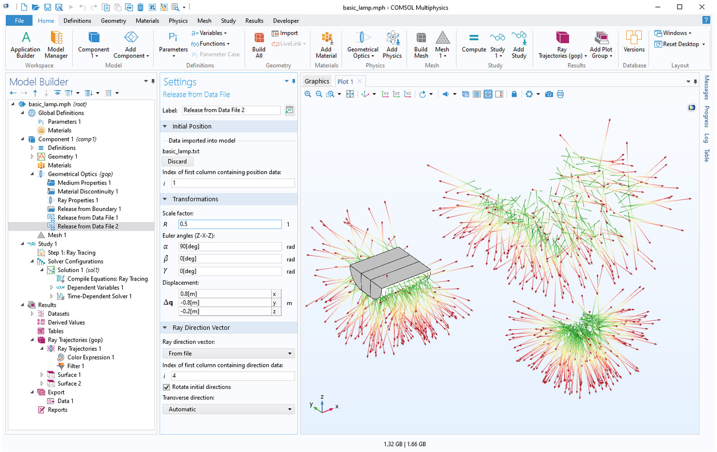
Transformations when Loading Ray Coordinates from a File
When you use the Release from Data File node to load the ray release positions from a file, you can now apply Transformations to the initial coordinates. You can use any combination of dilation (scaling), rotation, and translation. Optionally, if the initial ray direction is also loaded from a file, then you can apply the same rotation to both the position and direction.
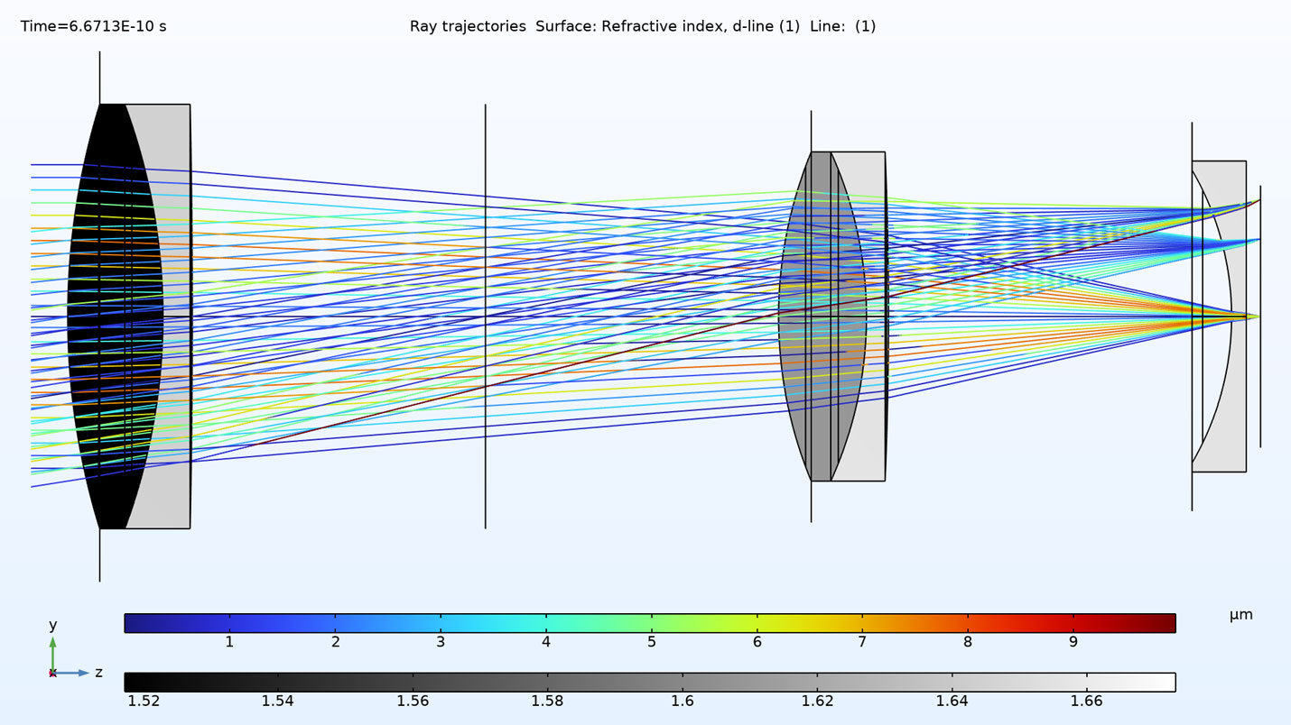
Easier Postprocessing of Refractive Index and Abbe Number
Built-in postprocessing variables are now available for the refractive index at the helium d-line, hydrogen F-line, and hydrogen C-line. The Abbe number is also defined. These built-in variables can be used in any plot type (such as Slice or Volume plots) to visualize the refractive index or dispersion of all optical glasses in a ray optics model. See these new postprocessing features in the existing Double Gauss Lens and Petzval Lens tutorial models.
Simplified Names for Nonlocal Couplings
The Geometrical Optics interface defines couplings to compute the sum, average, maximum, or minimum of an expression over the rays in a model. In this version, the names of these couplings have been simplified for easier use. View this change in the following existing models:
- Czerny-Turner Monochromator
- Petzval Lens Geometric Modulation Transfer Function
- Ray Release Based on a Plane Electromagnetic Wave
- Ray Release from a Dipole Antenna Source (2D Axisymmetric)
- Ray Release from a Dipole Antenna Source (3D)
The following table lists the old and new coupling names.
| Coupling Description | Old Name | New Name |
|---|---|---|
| Sum over rays | gop.gopop1(expr) | gop.sum(expr) |
| Sum over all rays | gop.gopop_all1(expr) | gop.sum_all(expr) |
| Average over rays | gop.gopaveop1(expr) | gop.ave(expr) |
| Average over all rays | gop.gopaveop_all1(expr) | gop.ave_all(expr) |
| Maximum over rays | gop.gopmaxop1(expr) | gop.max(expr) |
| Maximum over all rays | gop.gopmaxop_all1(expr) | gop.max_all(expr) |
| Minimum over rays | gop.gopminop1(expr) | gop.min(expr) |
| Minimum over all rays | gop.gopminop_all1(expr) | gop.min_all(expr) |
| Evaluate at maximum over rays | gop.gopmaxop1(expr, evalExpr) | gop.max(expr, evalExpr) |
| Evaluate at maximum over all rays | gop.gopmaxop_all1(expr, evalExpr) | gop.max_all(expr, evalExpr) |
| Evaluate at minimum over rays | gop.gopminop1(expr, evalExpr) | gop.min(expr, evalExpr) |
| Evaluate at minimum over all rays | gop.gopminop_all1(expr, evalExpr) | gop.min_all(expr, evalExpr) |
The old names will still work in version 6.0 as well, so it is not necessary to update any existing models.
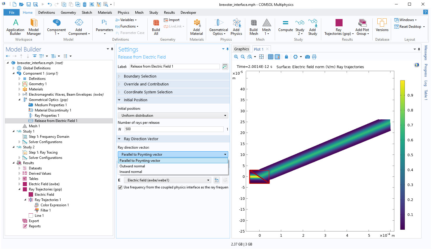
Release from Electric Field Improvement
It is now easier to release rays with initial intensity and polarization based on the full-wave FEM solution from an adjacent domain. When you use the Release from Electric Field node, the initial ray direction can now be taken directly from the Poynting vector of the field solved for in the adjacent domain.
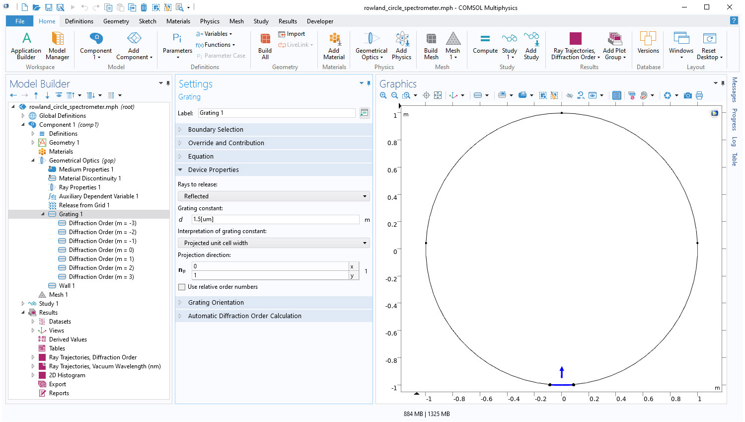
Improved Handling of Curved Gratings
The interpretation of the groove spacing in curved diffraction gratings is now much more transparent and more easily customizable. You can choose whether the specified grating constant should be interpreted as the distance between grooves on the grating surface (as it always was in version 5.6 and earlier), or whether the specified grating constant is actually the projected distance between grooves in a tangent plane. You can see this feature in the new Rowland Circle Spectrometer model.
New Tutorial Models
COMSOL Multiphysics® version 6.0 brings three new tutorial models to the Ray Optics Module.
Petzval Lens Optimization

Application Library Title:
petzval_lens_optimization
Download from the Application Gallery
Microlithography Lens
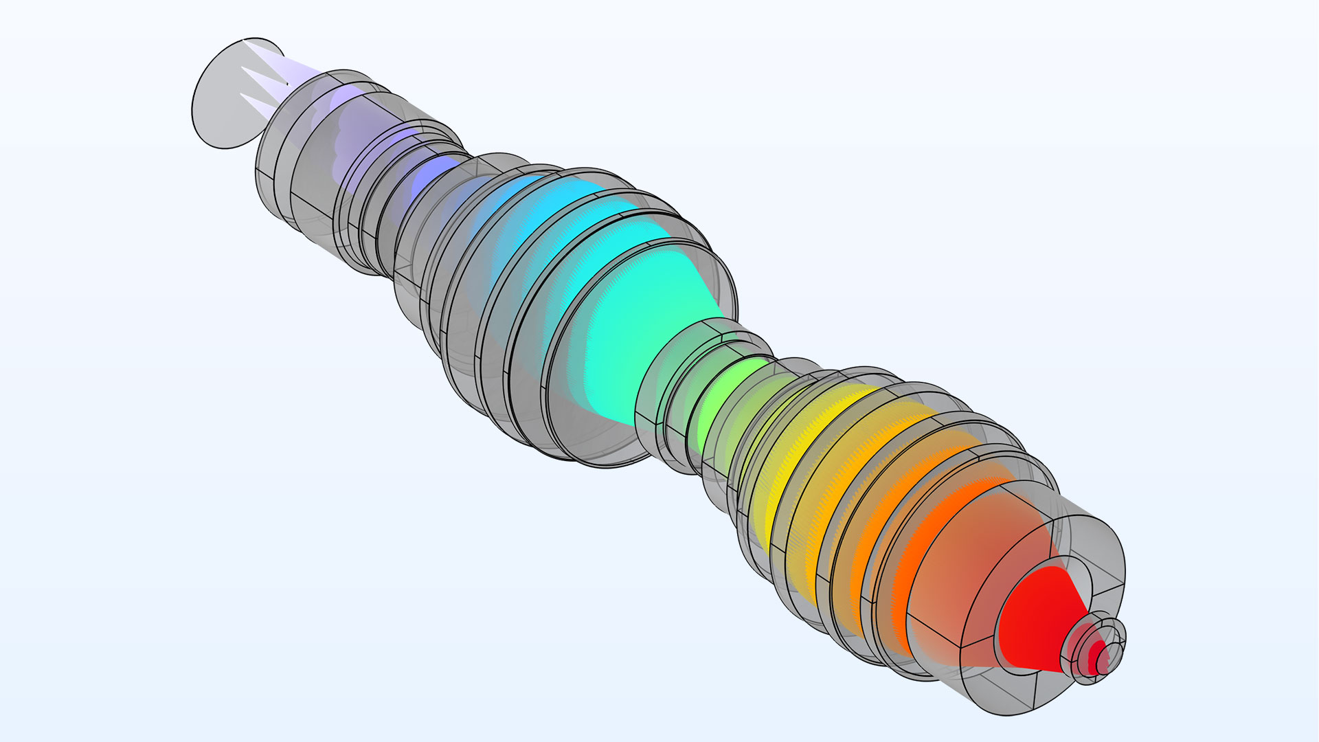
Application Library Title:
microlithography_lens
Download from the Application Gallery
Rowland Circle Spectrometer
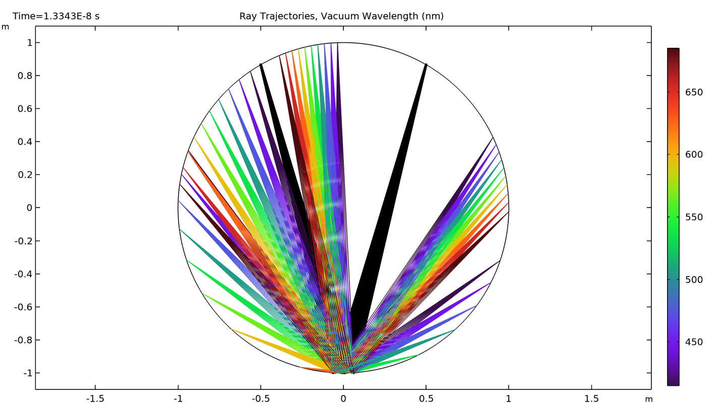
Application Library Title:
rowland_circle_spectrometer
Download from the Application Gallery