RF Module Updates
For users of the RF Module, COMSOL Multiphysics® version 6.0 introduces a new physics interface based on the boundary element method, a study step specializing in mesh adaptation, and new tutorial models analyzing coplanar waveguide (CPW) structures. Learn more about the news below.
Electromagnetic Wave, Boundary Elements
When modeling the scattering properties of objects, evaluating electric fields far from the scatterer, or far-fields of an antenna placed on an electrically large platform, the formulation based on the boundary element method (BEM) can improve the computation efficiency. The new physics interface called Electromagnetic Waves, Boundary Elements solves the vector Helmholtz equation for piecewise-constant material properties with the electric field as the dependent variable. BEM can be coupled to the finite element method (FEM), so-called hybrid BEM–FEM, to compute the field and interaction with other conductive objects outside the FEM domains. The new FEM–BEM Coupling of a Microstrip Patch Antenna tutorial model demonstrates this new interface.
Mesh Adaptation Study Step
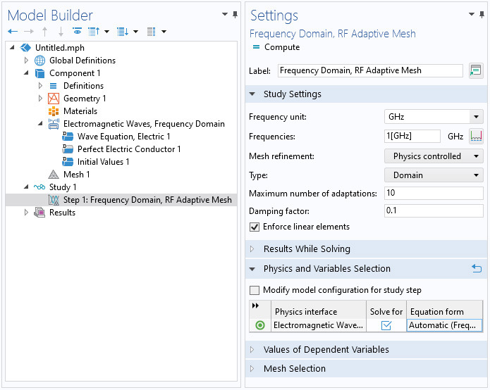
A new Frequency Domain, RF Adaptive Mesh study makes the workflow much easier when setting up mesh adaptation for modeling microwave and millimeter-wave antennas and circuits. This dedicated study step automatically provides the solver settings needed. For efficiency reasons, linear element discretization is used in the adaptive process. In a next step, a frequency sweep is typically used to characterize the device under test.
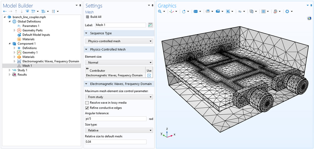
Enhanced Physics-Controlled Mesh on Conductive Edges
Strong electric fields tend to be confined around the edges of conductive boundaries. A finer mesh around these edges may help a simulation accurately analyze the resonance behavior of a device in the frequency domain. When using a physics-controlled mesh, a new Refine conductive edges option quickly identifies the exterior edges of signal path boundaries configured by perfect electric conductors or transition boundary conditions and applies the user-specified mesh size. This technique can be used as an alternative to adaptive meshing. You can see this new option in the existing Coplanar Waveguide Bandpass Filter tutorial model as well as two new tutorial models, Modeling of a CPW Using Numeric TEM Ports and Modeling of a Grounded CPW Using Numeric TEM Ports.
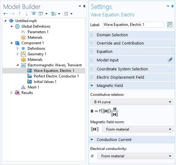
B-H Curve Magnetic Constitutive Relation
A new Constitutive relation option, B-H curve, has been added to model nonlinear magnetic phenomena. The material properties from the Nonlinear Magnetic Material Library, available with the RF Module, can be used to relate magnetic field and magnetic flux density. The B-H curve data from the material library are provided as interpolation functions for the magnetization curve without hysteresis effects. The effect of electrostatic discharge on a ferrite device can be studied to identify undesirable RF noise generation.
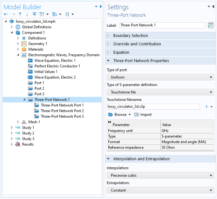
Three-Port Network
The Electromagnetic Waves, Frequency Domain interface now features a Three-Port Network boundary condition that characterizes the response of a three-port network component using S-parameters. You can import a Touchstone file to describe the physical behavior and response of a three-port device or system through three-port boundaries without addressing a complicated geometry.
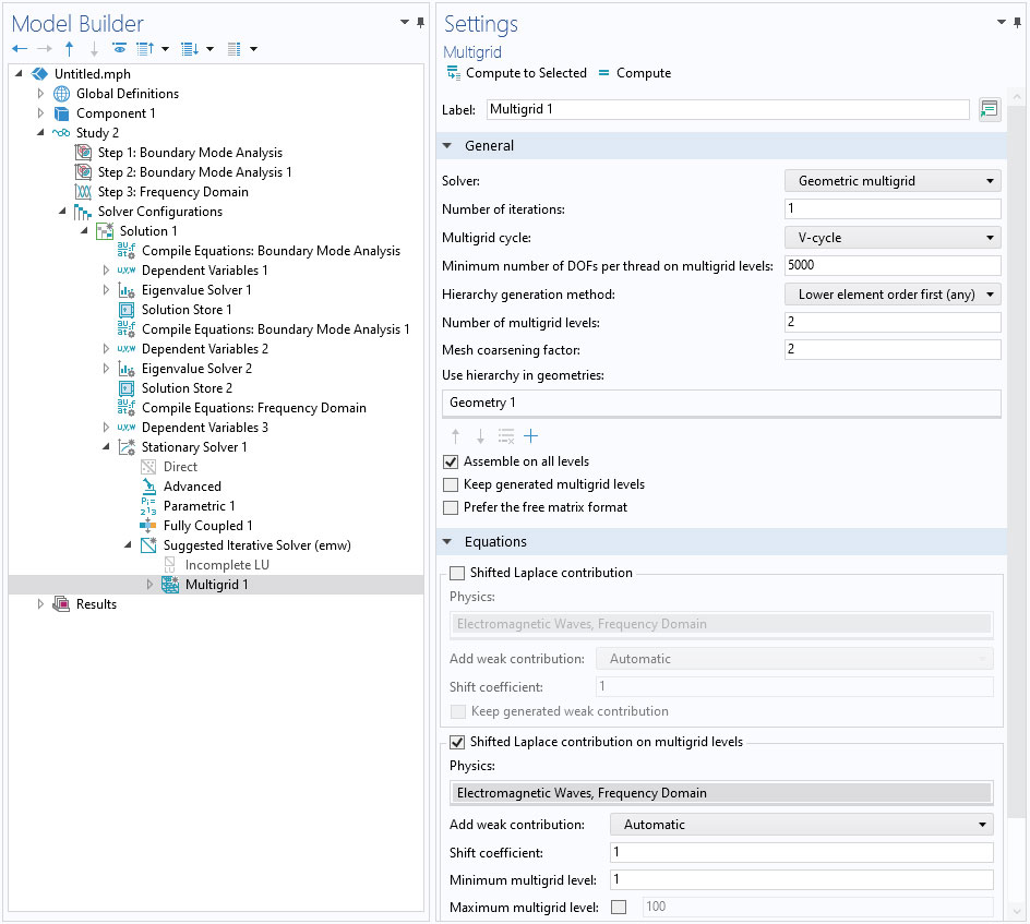
Shifted Laplace Contribution on Multigrid Levels
If no geometrical feature sizes are smaller than half a wavelength and the operating frequency is high, modeling with a higher-order element, such as cubic element discretization, is beneficial for faster computation. The computation efficiency can be further improved by selecting the Shifted Laplace contribution on multigrid levels check box under the Multigrid study settings.
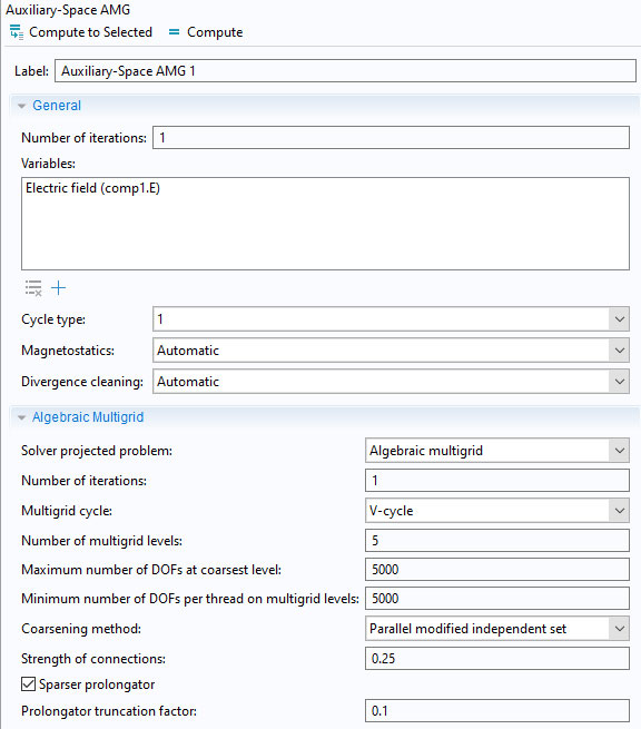
New Algebraic Multigrid Methods
The standard, or classical algebraic, multigrid method has been extended with a new coarsening method called Parallel modified independent set. This method supports cluster computing. Furthermore, the Auxiliary-Space AMG method has been extended to support complex-valued curl-element formulations.
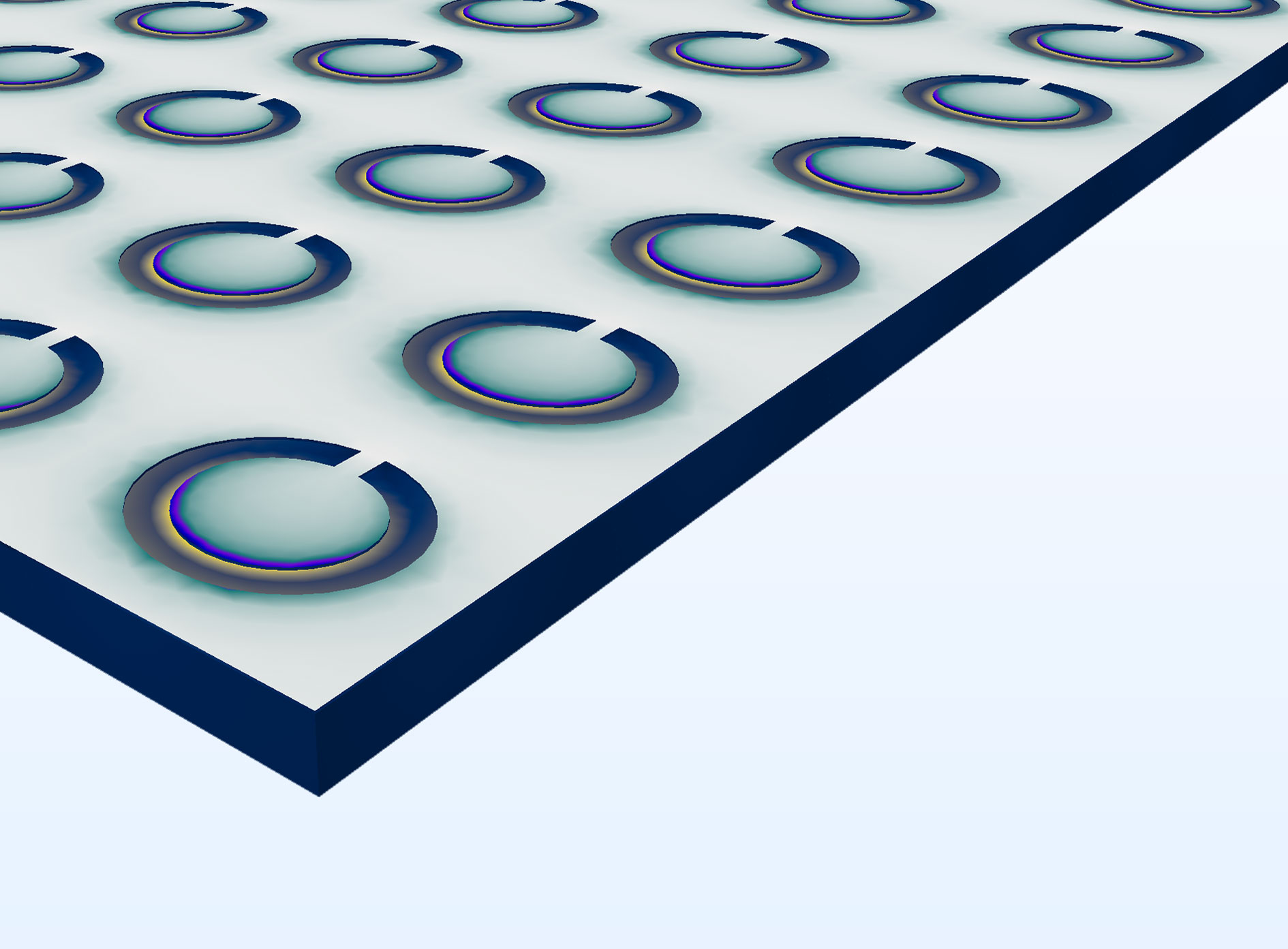
Iterative Solver Suggestion for Periodic Structures
Typical periodic problems are solved with a direct solver. However, the direct solver consumes a lot of memory when the periodic unit cell size is not subwavelength. In this case, switch to the Suggested Iterative Solver to finish the computation faster with less memory usage.
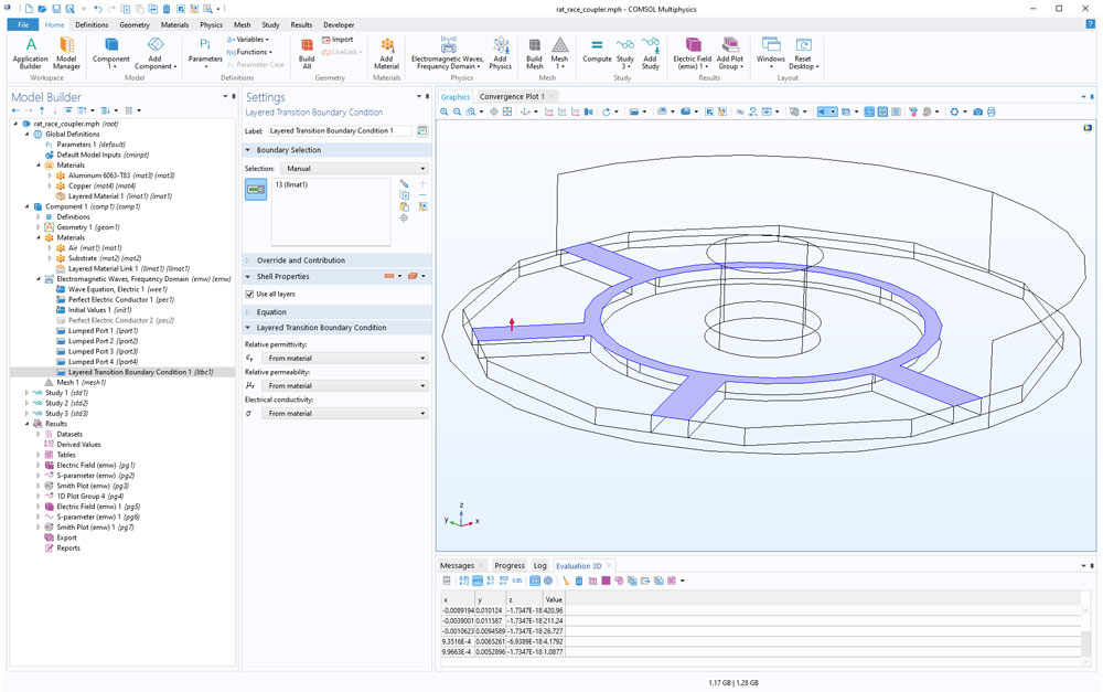
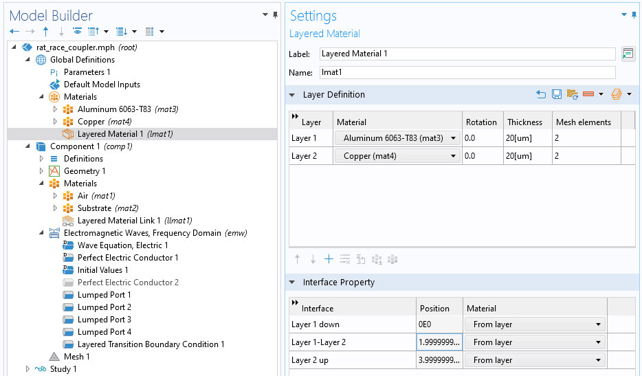
Layered Transition Boundary Condition
Multiple thin layers such as gold-plated copper of circuit board trace or close to normal incidence on an antireflection coating to an optical lens, can be described by the new Layered Transition Boundary Condition feature. It requires combining this boundary condition with the Layered Material feature in the global Materials, and Layered Material Link feature in the component Materials node. You can see this new feature demonstrated in the Rat-Race Coupler tutorial model.
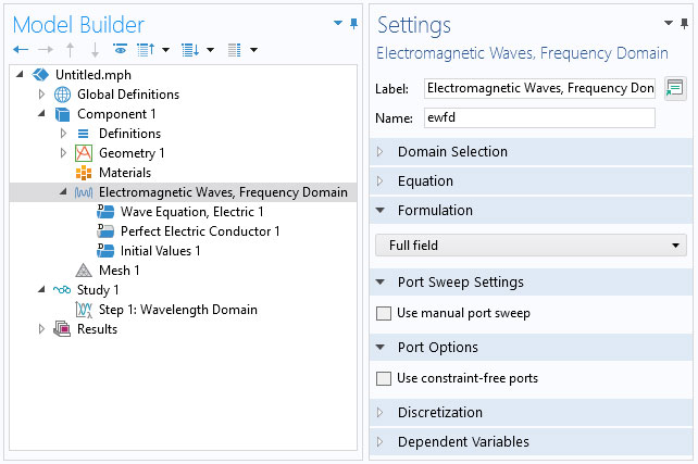
Constraint-Free Port Formulation
The Use constraint-free ports option is available to calculate the expansion coefficients as overlap integral, while in the default port formulation, the expansion coefficients (or S-parameters) are calculated by adding a scalar dependent variable for each coefficient and then adding a constraint to enforce the series expansion. This new option can be advantageous when using many ports, as no constraint elimination is required.
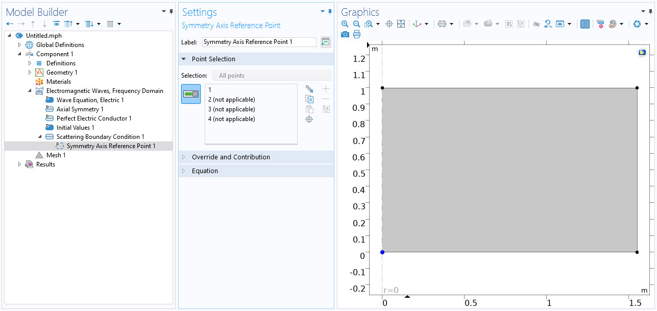
Symmetry Axis Reference Point
A new Symmetry Axis Reference Point feature helps to define Gaussian beam input fields in 2D axisymmetry. In the Scattering Boundary Condition or Matched Boundary Condition nodes, this is added as a default subnode when an incident field is defined. The Symmetry Axis Reference Point feature defines a reference position at the intersection point between the parent node's boundary selection and the symmetry axis.
Default Plots for Numeric Port Mode Fields
To simplify the inspection of the port mode fields, they are now automatically created when Numeric port types are used. You can see this default plot in the Modeling of a CPW Using Numeric TEM Ports and Waveguide Adapter tutorial models.
Reflection Coefficient with Multiple Excitation
When exciting all ports, as in a phased antenna array, it is possible to compute the reflection coefficient at each excited port that includes the impedance mismatching as well as coupling by adjacent active ports.
New and Updated Tutorial Models
COMSOL Multiphysics® version 6.0 brings several new and updated tutorial models to the RF Module.
Modeling of a CPW Using Numeric TEM Ports
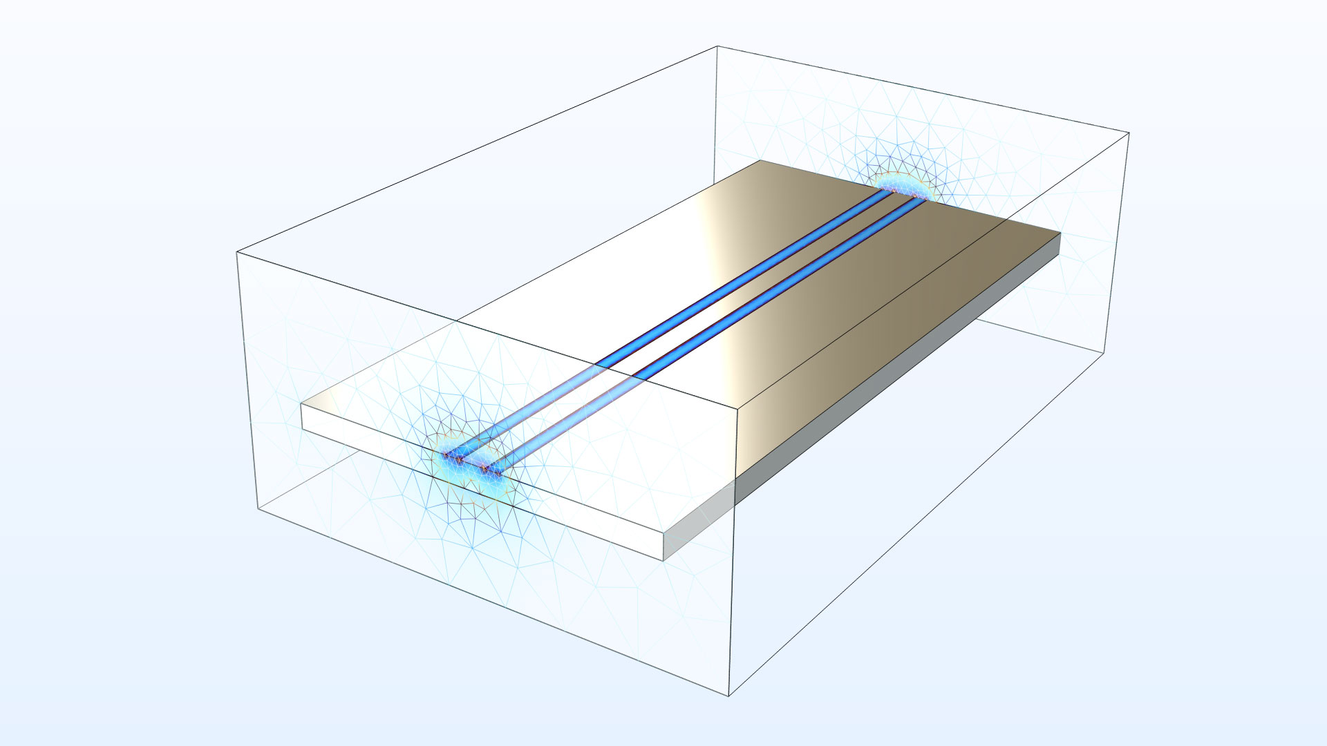
Application Library Title:
cpw_numeric_tem_port
Download from the Application Gallery
Modeling of a Grounded CPW Using Numeric TEM Ports
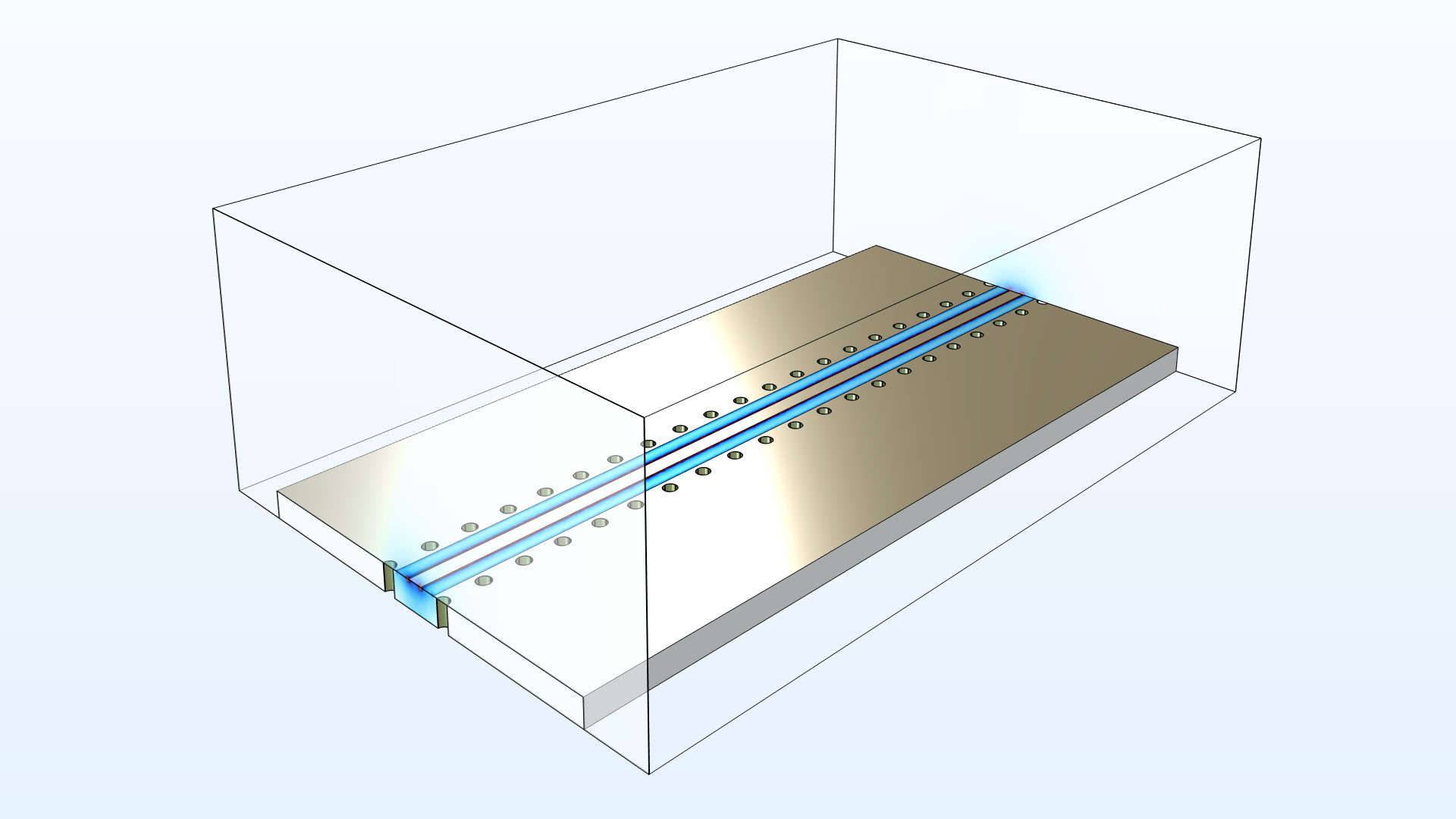
Application Library Title:
gcpw_numeric_tem_port
Download from the Application Gallery
FEM–BEM Coupling of a Microstrip Patch Antenna

Application Library Title:
microstrip_patch_antenna_fem_bem
Download from the Application Gallery
CPW Resonator for Circuit Quantum Electrodynamics
The coupled CPW resonator behaves like a high-Q bandstop filter. The tangential component of the electric field is plotted.
Application Library Title:
cpw_resonator
Download from the Application Gallery
Wi-Fi Booster Yagi–Uda Antenna

Application Library Title:
yagi_uda_antenna
Download from the Application Gallery