Modeling with PDEs: Multiphysics Systems of Equations
In Part 8 of this course on modeling with partial differential equations (PDEs), we will learn how to use the PDE interfaces to model systems of equations. As an example, we will use the Coefficient Form PDE interface to recreate the built-in functionality available in the Joule Heating multiphysics interface, available from the Model Wizard. Using the predefined multiphysics interface for Joule heating is, of course, much easier and quicker for this type of modeling compared to implementing this by hand. However, learning how to set up the corresponding equation system from scratch will prepare you for setting up more general systems, including systems that are not available as a built-in option in the COMSOL Multiphysics® software.
Modeling with Multiple Dependent Variables
All PDE interfaces and equation forms support the use of multiple dependent variables in a system of PDEs, which can be coupled in several different ways. For a complete description of what options are available for modeling systems of equations, see the COMSOL Multiphysics Reference Manual documentation, specifically the Multiple Dependent Variables — Equation Systems section of the chapter, Equation-Based Modeling.
There are several different types of equation systems that can be modeled using the equation-based, or Mathematics, interfaces. For example:
- When the variables represent different physics. One example of this is Joule heating where the dependent variables are the voltage,
 , and the temperature,
  .
. - When the variables represent the same physics. In such cases, the dependent variables frequently represent the components of a vector or tensor field, such as the displacement field components for structural mechanics.
- Combinations of 1 and 2.
In this article, we will look more closely at the case of Joule heating, a system of type 1, as mentioned here. In the next article we will study systems of type 2.
Joule Heating and Variables that Represent Different Physics
When the equation system represents Joule heating, the system of PDEs can be written as:


where  is the electric conductivity,
  is the density,
  is the heat capacity, and
  is the thermal conductivity. The first equation is that of conservation of currents. The second equation is the heat transfer equation with a Joule heating source term.
Note that the Joule heating source term can also be written as:

There are multiple ways of defining a Joule heating system of equations in COMSOL Multiphysics®. To learn more about using the built-in options, see our Learning Center course on defining multiphysics models.
As an alternative to using the built-in physics interfaces, you could instead define this system of equations using the Coefficient Form PDE interface, General Form PDE interface, or Weak Form PDE interface. Here, we will focus on using the Coefficient Form PDE interface. For this, we can use what we learned in the Learning Center article on modeling with PDEs for diffusion-type equations.
We can identify the first equation as Poisson's equation. This means that for the stationary version of Coefficient Form PDE:

we can identify the coefficients as:


and all other coefficients are zero. For the heat equation

we need to compare with the transient version of Coefficient Form PDE:

we see that:


Using Coefficient Form PDE, there are two ways of entering this equation system: as a system of two scalar Coefficient Form PDE interfaces or as a system of one vector-valued Coefficient Form PDE interface with two vector components, and .
Joule Heating as a System of Two Scalar Coefficient Form PDE Interfaces
Using two scalar Coefficient Form PDE interfaces is very similar to using predefined physics interfaces. Start by adding a Coefficient Form PDE interface, where we have changed Field name and Dependent variables to V.
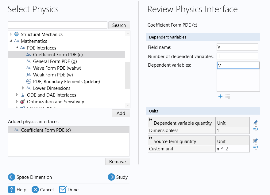
The Select Physics window, where the Coefficient Form PDE interface has been added to the model.
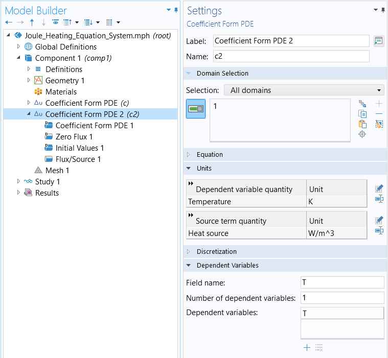
Next, add another Coefficient Form PDE interface with both Field name and Dependent variables set to T.
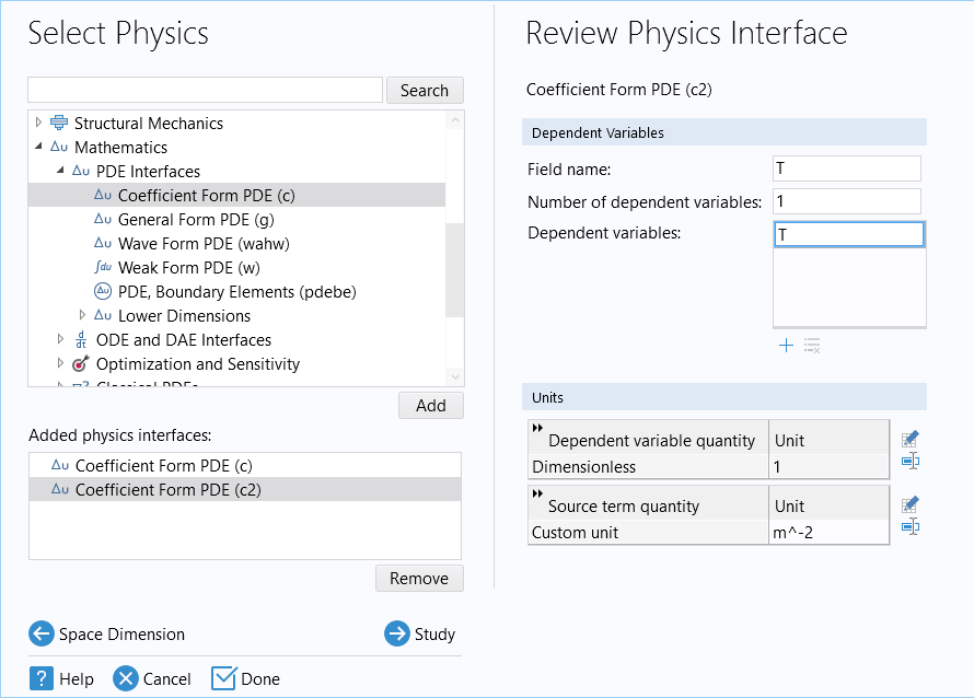
A second Coefficient Form PDE interface added through the Model Wizard.
In this case, there is no reason to have different names for Field name and Dependent variables. However, if we create a vector-valued system of equations, then we can use Field name as a reference for a vector of dependent variables.
In the next step, select a Time-Dependent study. The Model Builder tree appears as follows:
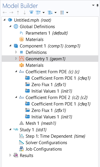
The model tree after adding the physics interfaces and study through the Model Wizard.
For this example, we will use a simple conductive block that is 1-by-0.1-by-0.01 mm, having a boundary condition of 1 V on one side and 0 V (or ground) on the other side.
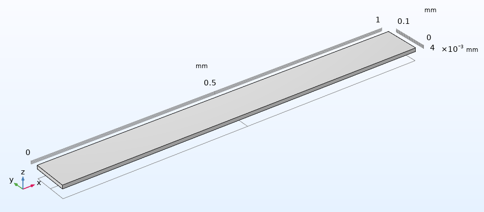
The model geometry for a simple conductive block.
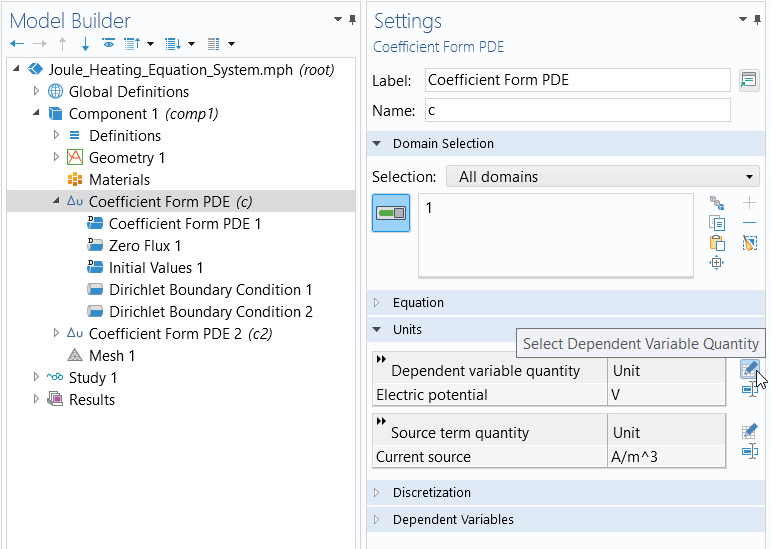
Choosing Units
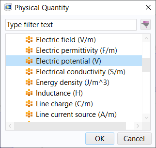
In the Settings window for the Coefficient Form PDE interface, change the units for the Dependent variable quantity to Electric potential (V) and the Source term quantity to Current source (A/m^3).
The settings for the first Coefficient Form PDE interface.
You can do this by clicking the respective icon (pictured below) that opens the Physical Quantity dialog box. From there, you can select the appropriate quantities.
 The Physical Quantity box with Electric potential (V) highlighted.
 The Physical Quantity box with Current source (A/m^3) highlighted.
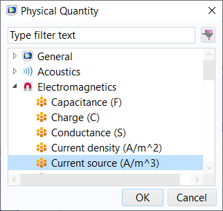
 The Physical Quantity box with Dimensionless (1) highlighted.
If you do not want to work with units, you can select the Dimensionless option in the General section of the Physical Quantity dialog box.
Conservation of Currents
If we assume an electric conductivity  , corresponding to a moderately conductive material, then the Coefficient Form PDE node settings are as follows:
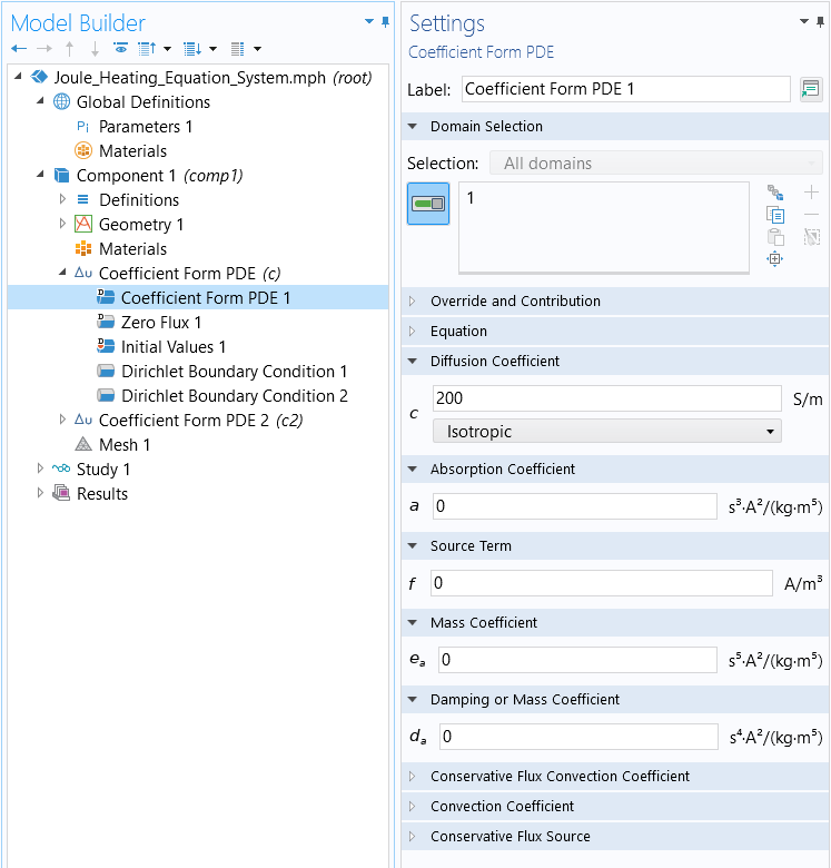
The settings for the Coefficient Form PDE node.
Using a Dirichlet Boundary Condition, set the voltage to 1 V on the left boundary. Similarly, we can add a second Dirichlet Boundary Condition for the boundary on the right end with the voltage equal to 0 V, corresponding to ground.
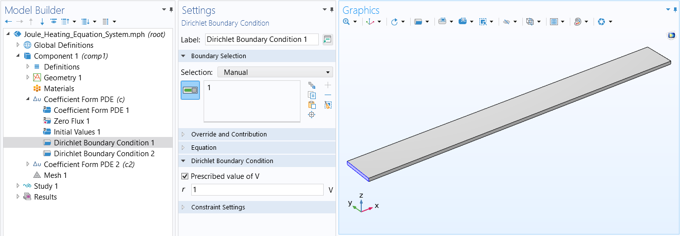 The Model Builder with the Dirichlet Boundary Condition selected, the corresponding Settings window, and the Graphics window with the conductive block model.
The settings for the Dirichlet Boundary Condition.
Heat Transfer
In the Settings window for the second interface, Coefficient Form PDE 2, change the units to Temperature (K) for the Dependent variable quantity and Heat source (W/m^3) for the Source term quantity.
The settings for the second Coefficient Form PDE interface.
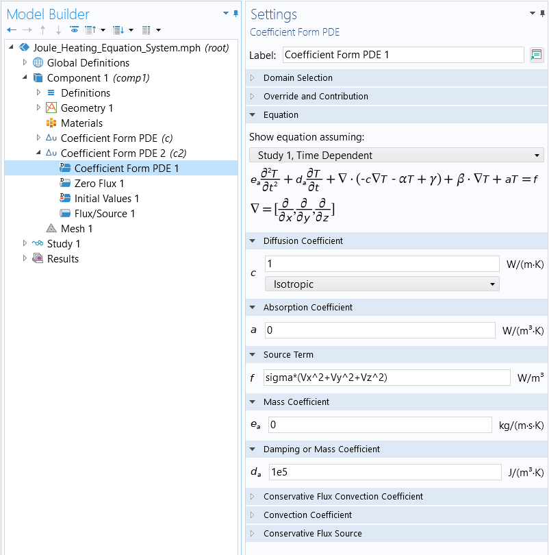
Using the electric conductivity and further assuming  and
and  , the Coefficient Form PDE node settings for the second equation are as follows:
The settings for the Coefficient Form PDE node for the second equation.
where the source term corresponds to
 .
.
In the software, the derivative components of a dependent variable, up to derivatives of the second order, are always available as expressions for dependent variable names, with the spatial components appended. If the dependent variable is V, then the derivative components are available as Vx, Vy, Vz, Vxx, Vxy, and so on.
For the second equation, for all boundaries, use a Flux/Source boundary condition:

with the coefficient  and
and  . This boundary condition means that the boundaries are being cooled at a rate that is proportional to the temperature difference of the surroundings. Note that this boundary condition can equivalently be implemented by setting
  and
and  .
.
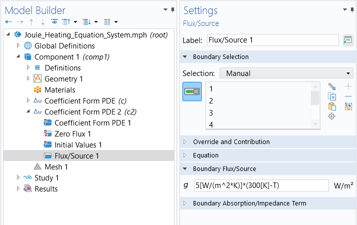
The settings for the Flux/Source boundary condition.
The second equation has a time-derivative term and therefore requires updating the values for the Initial Values node. We will assume that the device is at 300 K at time t = 0. Since this PDE only has a first-order time derivative, we do not need to worry about the initial condition for

The settings for the Initial Values node.
Results
Now, run Study 1 using the default settings for the Output times between 0 and 1 seconds with results output for every 0.1 seconds.
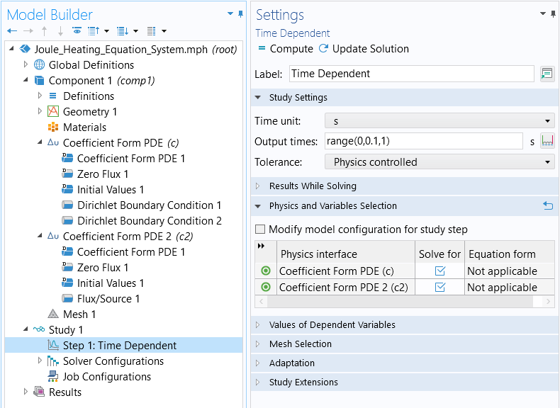
The settings for the time dependent study performed.
The result is a temperature of around 480 K at around 1 second.
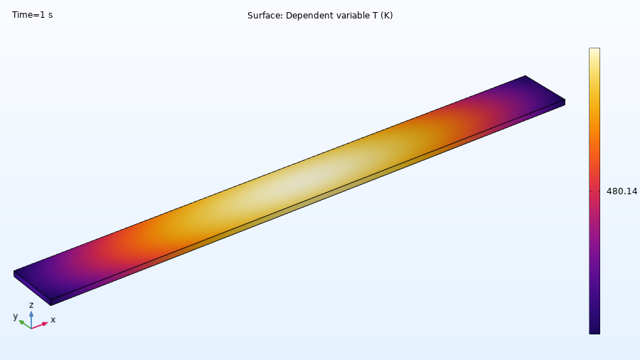
Results for the temperature distribution of the block.
We can also plot the voltage drop across the object.
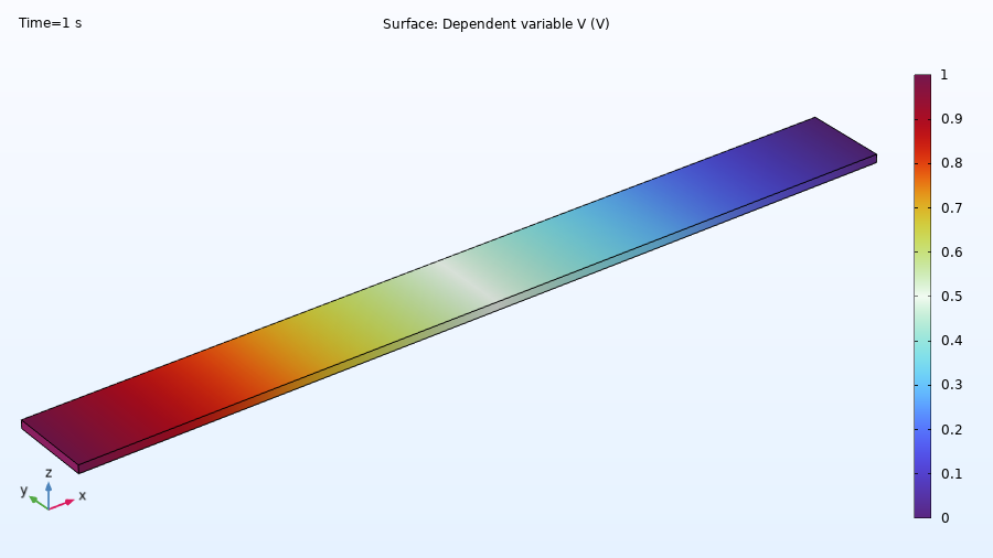
Results for the electric potential of the block.
You can now define variables for quantities, such as the electric field or current density, and then use them in expressions.
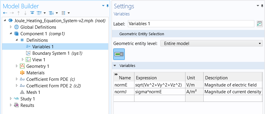
The variables defined after computing the study.
After solving again, we can, for example, visualize the variable normJ in a plot.
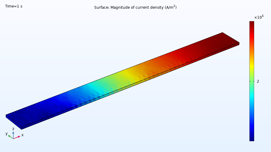
Results for the magnitude of current density of the block.
Further Learning
Although the model used throughout this article is available for download, we encourage you to first build the model yourself by following the guidance provided here. Thereafter, you can open and explore the model file. This will reinforce how to set up equation systems from scratch.
Submit feedback about this page or contact support here.