Die Application Gallery bietet COMSOL Multiphysics® Tutorial- und Demo-App-Dateien, die für die Bereiche Elektromagnetik, Strukturmechanik, Akustik, Strömung, Wärmetransport und Chemie relevant sind. Sie können diese Beispiele als Ausgangspunkt für Ihre eigene Simulationsarbeit verwenden, indem Sie das Tutorial-Modell oder die Demo-App-Datei und die dazugehörigen Anleitungen herunterladen.
Suchen Sie über die Schnellsuche nach Tutorials und Apps, die für Ihr Fachgebiet relevant sind. Beachten Sie, dass viele der hier vorgestellten Beispiele auch über die Application Libraries zugänglich sind, die in die COMSOL Multiphysics® Software integriert und über das Menü File verfügbar sind.

This example models the desalination of water by capacitive deionization in a "flow-between" cell (fbCDI). The model geometry is in 2D. Steady Brinkman flow, a tertiary current distribution, and the improved modified Donnan description of the deionization process is assumed. Mehr lesen

This model shows how to control the position of the base of an inverted pendulum to keep it vertical. The control is performed using a PID controller in Simulink®. The position of the base is constrained within specified limits, and an external force is applied at the base to keep it ... Mehr lesen

The present example simulates the turbulent flow over a 3D hill geometry using the Large Eddy Simulation (LES) interface with synthetic turbulence at the inlet boundary. Mehr lesen

This model computes the fundamental eigenfrequency and eigenmode for a tuning fork that is synchronized from SOLIDWORKS® via the LiveLink™ interface. The length of the fork is then optimized so that the tuning fork sounds the note A, 440 Hz. Mehr lesen

This model computes the fundamental eigenfrequency and eigenmode for a tuning fork that is synchronized from Solid Edge® via the LiveLink™ interface. The length of the fork is then optimized so that the tuning fork sounds the note A, 440 Hz. Mehr lesen
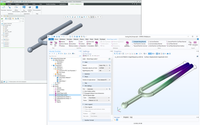
This model computes the fundamental eigenfrequency and eigenmode for a tuning fork that is synchronized from PTC Creo Parametric™ via the LiveLink™ interface. The length of the fork is then optimized so that the tuning fork sounds the note A, 440 Hz. Mehr lesen

This example shows how to compute deformations caused by secondary creep in a turbine stator blade. The creep rate is highly influenced by temperature, and the deformation and stress relaxation is thus controlled by the temperature field. Mehr lesen

In this example, phase transformation data and phase material properties are imported from JMatPro, and used to compute CCT curves. Dilatometry curves (axial thermal strain) are computed across a range of cooling rates. Mehr lesen

This tutorial model shows the setup of a 2D axisymmetric stress analysis, through contact, of a 3D threaded pipe fitting. The example involves synchronizing the 3D Solid Edge® geometry and selections, which specify the faces in contact, with the 2D geometry in COMSOL ... Mehr lesen
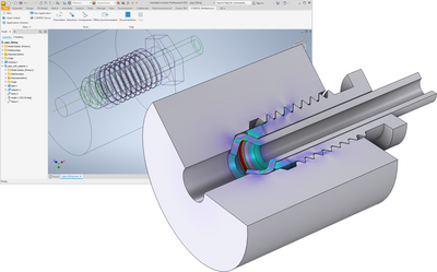
This tutorial model shows the setup of a 2D axisymmetric stress analysis, through contact, of a 3D threaded pipe fitting. The example involves synchronizing the 3D Inventor® geometry and selections, which specify the faces in contact, with the 2D geometry in COMSOL Multiphysics ... Mehr lesen