

The trajectories of particles through fields can often be modeled using a one-way coupling between physics interfaces. In other words, we can first compute the fields, such as an electric field, magnetic field, or fluid velocity field, and then use these fields to exert forces on the particles using the Particle Tracing Module. If the number density of the particles is very large, however, the particles begin to noticeably perturb the fields around them, and a two-way coupling is needed — that is, the fields affect the motion of the particles, and the particle trajectories affect the fields. For example, charged particles act as point sources that affect the electric field around them, and small particles that move through a fluid may drag the fluid with them. Although two-way coupling between particles and fields presents new modeling challenges and is computationally more time consuming than one-way coupling, new tools available in COMSOL version 4.4 can address many of these challenges by using an efficient, self-consistent approach.
One-Way vs. Two-Way Coupling
Consider the motion of a group of ions or electrons through electric and magnetic fields. To model the system using a one-way coupling, we first solve for the electric and magnetic fields, typically using a stationary or frequency-domain study step. To compute the trajectories of charged particles in these fields, we can then use the Charged Particle Tracing interface, which solves a second-order ODE for each particle’s position:
Here, m\mathbf{v} is the particle’s momentum, q is the particle’s charge, \mathbf{E} is the electric field, and \mathbf{B} is the magnetic flux density. This approach relies on the following assumptions:
- The fields are either stationary, change very slowly relative to the motion of the particles, or vary sinusoidally over time.
- The charged particles have a negligibly small effect on the electric and magnetic fields.
Being able to compute the fields using a stationary or frequency-domain study step is a tremendous time saver, since time-dependent studies involving the Particle Tracing Module often require a very large number of time steps. Several examples of one-way coupling between particles and electromagnetic fields are available in the Model Gallery, including the following:
- Magnetic Lens (requires the AC/DC Module)
- Particle Tracing in a Quadrupole Mass Spectrometer (requires the AC/DC Module)
- Quadrupole Mass Filter (requires the AC/DC Module)
- Einzel Lens
Several examples of one-way coupling between fluid velocity fields and particle trajectories are also available, such as the following:
All of these examples follow the same pattern: compute the field using a stationary or frequency-domain study step, then couple the solution to a time-dependent study step for the particle trajectories.
If the particles are numerous enough that they noticeably affect fields in the surrounding domains, we must recompute the fields at each time step to account for the changed positions of the particles. At this point, a two-way coupling between particles and fields is required. Typical examples of systems requiring a two-way coupling are ion and electron beams, electron guns, and sprays of particles entering a crossflow. In these situations, we must often compute the space charge density due to a group of charged particles or the volume force exerted by particles on a fluid.
Implementing Point Sources
The particles used in the physics interfaces of the Particle Tracing Module are treated as point masses in many respects. Although some pre-defined forces, such as the drag force, are size-dependent, the particles are considered infinitesimally small for the purpose of determining when they collide with walls. In addition, particles immersed in a fluid don’t displace any volume of fluid. Because each particle is treated as a point mass, the charge density or volume force due to the presence of a particle reaches a singularity at that particle’s location.
In some instances, you can improve the accuracy of a solution close to a singularity using adaptive mesh refinement; see, for example, Implementing a Point Source Using Poisson’s Equation in the Model Gallery. However, this is not a viable option for managing singularities due to particles for several reasons: there can be a very large number of singularities, the particles are constantly moving, and they generally don’t coincide with nodes of the finite element mesh. Instead, the singularities are avoided by distributing the space charge density or volume force due to each particle over the mesh element the particle is currently in. Although this means that the solution is somewhat mesh-dependent, the error introduced is typically very small if the number of particles is sufficiently large.
Modeling Steady-State Systems
In the context of particle-field or fluid-particle interactions, we take steady-state to mean that the fields do not change over time. For example, an ion beam would be considered to operate under steady-state conditions if the electric field at any point remains constant, typically as a result of a constant ion flux. A pulsed beam, on the other hand, would not be considered a steady-state system.
A unique feature of steady-state systems is that they allow the particle trajectories and fields to be computed using a self-consistent method that is more efficient than computing the entire solution with a time-dependent study. This method involves the set-up of an iterative loop of different solver types, as we will see in the following example.
Creating a Self-Consistent Model of an Electron Beam with COMSOL 4.4
To illustrate the available solution techniques for steady-state systems with two-way coupling between particles and fields, consider a beam of electrons that is released into a large, open area at constant user-defined current. In order to model a large, open area, we add an Infinite Element Domain around the exterior of the modeling domain, represented by the highlighted areas in the image below. The circle shown at one end of the cylinder will be used to define an Inlet feature for electrons.

We expect that the electrons in the beam will repel each other, causing the beam to become wider as it propagates forward. We will assume that the electrons are non-relativistic, so that the force on the beam electrons due to the beam’s magnetic field is negligibly small compared to the force due to the beam’s electric field. We seek a self-consistent solution to the following equations of motion:
-\nabla \cdot \epsilon_0 \nabla V &= \sum_{i=1}^N q\delta \left({\mathbf{r}}-{\mathbf{q}}_i\right)\\
\frac{d}{dt}\left(m{\mathbf{v}}\right) &= -q\nabla V
\end{aligned}
The first equation is a Poisson equation for the electric potential, with a space charge density term due to the presence of charged particles. Here, \delta is the Dirac delta function, N is the total number of particles, \mathbf{r} is the position vector of a point in space, and \mathbf{q}_i is the position of the ith particle. The second equation is the equation of motion of a particle subjected to an electric force. Solving both equations of motion in the same time-dependent study would be extremely time consuming, and would require a very large number of particles to be released at small, regular time intervals to ensure that the desired beam current is maintained.
An alternative solution method involves a physics interface property called the Release type, available for the Charged Particle Tracing and Particle Tracing for Fluid Flow interfaces in COMSOL 4.4. The default setting, Transient, is the correct choice for most applications. Changing the Release type to “Static” affects the available settings of particle release features, such as the Inlet, and changes the way the Particle-Field Interaction and Fluid-Particle Interaction features work.

Working with the Static release type requires us to change our interpretation of what the model particles represent. Rather than representing a single particle or group of particles at a specific point in space, each model particle now represents a certain number of particles per unit time. The number of real particles per unit time represented by each model particle is computed so that each Inlet, Release, or Release from Grid feature provides a user-defined charged particle current or mass flow rate (for the Charged Particle Tracing and Particle Tracing for Fluid Flow interfaces, respectively).
To accompany this new interpretation of the model particles, the space charge density, \rho, due to the presence of charged particles is now computed as:
Here, f_{\textrm{rel}} is the number of ions or electrons per second represented by each model particle so that the user-defined current is obtained. Similarly, when modeling fluid-particle interactions, the volume force, \mathbf{F}_V, that is exerted by particles on the fluid is computed as:
where {\mathbf{F}}_{\textrm{D}} is the drag force on the particle. The time derivative on the left-hand side of each equation indicates that instead of creating a contribution to the space charge density at one location in space, each model particle leaves a trail of space charge or volume force along its trajectory, representing the combined effect of all particles that follow that trajectory. As a result, only a single release of model particles at time t=0 is needed to compute the space charge density due to an electron beam operating at constant current.
When computing the space charge density due to a group of particles, a time-dependent solver with a fixed maximum time step is recommended. The maximum time step should be small enough so that, on average, each particle spends several time steps inside each mesh element. In addition, the number of model particles should be large compared to the number of mesh elements in a cross section of the beam. These two guidelines ensure that the particles don’t “miss” any elements inside the beam, thereby creating non-physical gaps in the space charge distribution.
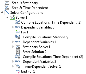
Creating a Solver Loop
So far, we’ve seen that a single release of particles can be used to compute the space charge density due to a continuous beam of charged particles. However, the resulting space charge density must still be coupled back to a Poisson equation for the electric potential. Changes to the electric potential might in turn perturb the particle trajectories. To reach a self-consistent solution, we can compute the electric potential using a stationary solver, then use this potential to compute the particle trajectories and space charge density using a time-dependent solver, then use the space charge density to recompute the electric potential, and so on. This type of iterative sequence can be implemented in COMSOL by adding For and End For nodes to the solver sequence. Any solvers in-between these two nodes will be executed a number of times specified by the user in the For node settings. New to COMSOL Multiphysics in version 4.4, the For and End For nodes give the user sophisticated tools to set up two-way coupling between physics interfaces that require different types of solvers.
The self-consistent solution confirms our expectations: the electron beam diverges due to its self potential. In the image below, the lines represent particle trajectories that begin in the background and move to the foreground. The shading of each line represents the model particle’s radial displacement from its original position; the slice plot shows the beam potential; and the arrows show the electric force acting on the beam due to self potential. The result is in close agreement with analytical expressions for the shape of a non-relativistic charged particle beam.

Although the method outlined above is only valid for static fields, it reduces the number of particles required for accurate modeling by several orders of magnitude. The Electron Beam Diverging Due to Self Potential model demonstrates the new For and End For nodes that can be added to the solver sequence with COMSOL 4.4.
Concluding Thoughts
- If the number density of particles is very low, the particles may have a negligibly small effect on electric, magnetic, or fluid velocity fields in the surrounding domain. In this case, computing the field first and then using this field to exert a force on the particles is the most efficient approach.
- To accurately model two-way coupling between particles and fields, use a large number of model particles and specify a fixed maximum time step. You may need to increase the number of particles or reduce the time step further after refining the mesh.
- The Static release type can be used to model a constant charged particle current or mass flow rate.
- If the field is not time-dependent, computing the fields and particle trajectories in separate steps within a solver loop can be much more efficient than including all physics in a single time-dependent study step.


Comments (3)
Euler Integral
December 5, 2013Cool new features, but it’s also possible to implement relativistic charged particles in vacuum space and see the power radiated at infinity? Without the need to use Liénard–Wiechert potential or retarded time whatsoever?
Thanks
Christopher Boucher
December 9, 2013Currently there is no built-in functionality for computing the power radiated by individual relativistic particles. The method described in this blog post is only appropriate for those cases in which the fields are not time-dependent. There is no need to analytically compute the Liénard-Wiechert potential at the point of observation in such cases.
Matteo Duranti
February 15, 2015I would like to some study for an idea I had. The fields (electric and magnetic) emitted by a single relativistic particle are still not simulated? Or now (2015, COMSOL 5) the situation is different?
Thanks