
As of version 5.3 of the COMSOL Multiphysics® software, the Subsurface Flow Module includes useful new features that enable you to set up complex modeling tasks more efficiently. For example, when modeling wells, meshing is significantly easier and is more intuitive to set up with the Well feature. In this blog post, we look at the Well feature, discussing how to use it and ways it enhances the modeling process.
Modeling Wells in COMSOL Multiphysics®
Modeling subsurface flow problems often deals with large modeling domains that are exposed to sources or sinks of a comparatively small size.
Previously, wells were introduced in COMSOL Multiphysics as small 3D cylinders in a large layered subsurface domain, as shown in this blog post about coupling heat transfer and porous media flow in a geothermal doublet. This approach was necessary to apply suitable boundary conditions and involved meshing small objects.
With the Well boundary condition — new in COMSOL Multiphysics 5.3 — the cylinders can be replaced by edges, which is better for the meshing algorithm and requires less meshing. The highlight of this feature is that it provides accurate solutions compared to resolving details explicitly. Let’s discuss the Well boundary condition in more detail.
The Settings for the Well Boundary Condition
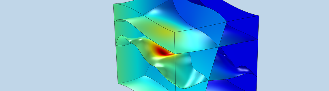
We first want to get familiar with the new boundary condition and its settings. The Well boundary condition is available as a Point feature in 2D and an Edge feature in 3D and can be used with the Darcy’s Law, Richards’ Equation and Two-Phase Darcy’s Law interfaces. With this boundary condition, you can choose whether the well is an injection or production well and specify either the pressure or mass flow. The images below show some of the different options that are available.

The settings for the modeling of an injection well with the Darcy’s Law, Richards’ Equation interface (left) and the Two-Phase Darcy’s Law interface (right), where the saturation must also be specified.
Comparing Two Approaches for Modeling Wells
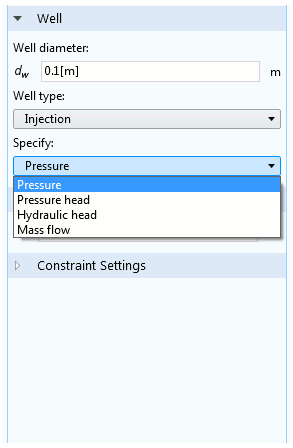
Let’s now see how the Well boundary condition compares with other options for modeling wells. For illustration purposes, we use a basic model, as shown in the image below.
Model geometry of a well with a radius of 0.5 m in a reservoir that has a radius of 20 m, height of 3 m, and is surrounded by an infinite elements domain.
Infinite elements are used so that we can apply a pressure at a large distance from the well without increasing the modeling domain. The geometry shown here resolves the well as a cylindrical surface. To be able to apply a boundary condition, the well cylinder must be cut out of the reservoir. Alternatively, a Mass Flux edge condition can be used — but only if we want to apply a mass flux, not a pressure. As of COMSOL Multiphysics 5.3, the Well boundary condition is available, which is suitable for pressure as well as mass flux conditions.
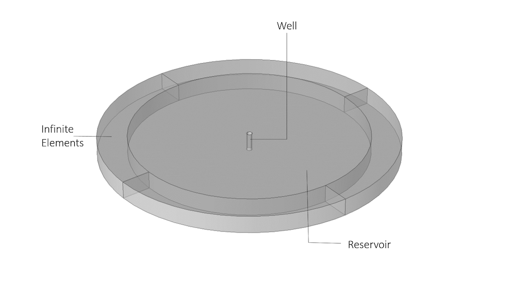
We compare the mesh in the two cases using exactly the same mesh settings. Here, we have 65,674 domain elements for the case where the well is fully resolved versus 28,728 domain elements when using the Well boundary condition. That is less than half the number of mesh elements.
Comparison of the mesh using the same settings between the case with a fully resolved well and when the Well boundary condition is used.
This advantage is only useful if we get an accurate solution. Continuing with this test case, we apply a mass flow rate, M0, of 1 kg/s at the well. This corresponds to a mass flux, N0, at the boundary with area, A, of . The mass flux at the edge of length, l, is
. The pressure is fixed at the outer infinite element boundaries.
A 1D plot of the pressure along the centerline shows almost perfect agreement with the approaches outside of the well.
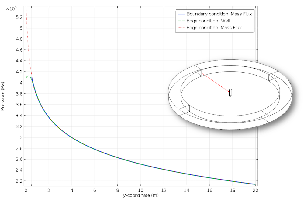
Comparison of the pressure along a cut line.
In contrast to specifying the mass flux on the edge, the Well feature accounts for the well radius, even if it is not resolved explicitly. To evaluate the pressure at the well, the Mass Flux edge feature is not suitable, since the expansion in the radial direction is not considered. The Well boundary condition provides a variable, dl.well1.p, which gives the well pressure.
Application of Coupled Heat Transfer and Porous Media Flow: Geothermal Doublet
The Well boundary condition can be used in the geothermal doublet example mentioned earlier. We use a slightly modified version of the model that is featured in the previous blog post. In this case, geothermal groundwater is produced through the production well at a rate of 150 l/s. The water is reinjected at the same rate after it has been used for heat generation with a temperature of 5°C. A horizontal hydraulic gradient of 2 mm/m is applied at the outer boundaries.
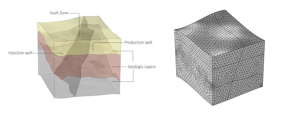
Model setup (left) and mesh (right) of the geothermal doublet model.
Prior to COMSOL Multiphysics 5.3, the production and injection wells were drawn as cylinders embedded in the geological formations, and the mass and heat fluxes were defined on the cylinders’ surfaces by using Inlet and Outlet boundary conditions for Darcy’s law and Temperature and Outflow boundary conditions for heat transfer.
Now, the wells are defined by single edges, and the new Well and Line Heat Source features are used for defining the mass and heat fluxes. The settings for both features are shown below.
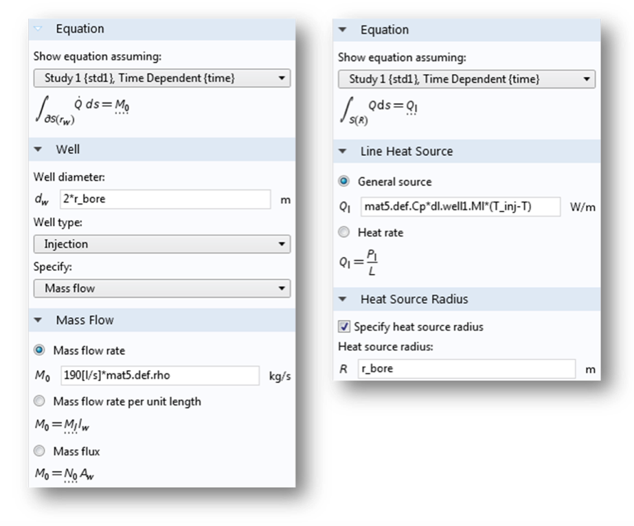
The settings for the Well (left) and Line Heat Source features (right).
In the Well feature, you specify the mass flow rate at the injection well by setting M0 = 150 l/s ρwater. The density of water is specified in the Materials node, which is accessed by the expression mat5.def.rho. For the line heat source, we define the source term per unit length according to Ql = MlCpΔT. Here, Ml is the mass flow rate per unit length and is automatically calculated by the Well feature (dl.well1.Ml); Cp is the specific heat capacity of water ( mat5.def.Cp); and ΔT = Tinj – T is the temperature difference between the injection temperature and the actual temperature.
With the Well feature, there are about 8% fewer mesh elements (118,000 versus 126,000) as compared to the model that uses cylinders as boreholes; and the simulation runs approximately 10% faster (31 minutes versus 26 minutes). The animation below shows the evolution of the temperature over 5 years.
The evolution of temperature in the geothermal reservoir over five years.
To prove that the Well feature gives the same results as the corresponding boundary condition on a cylindrical surface, we compare the results of the production temperature. We can see that there is very good agreement between the results.
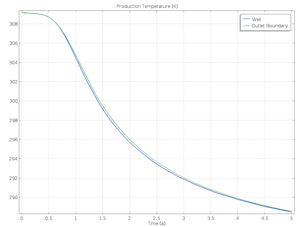
Comparison of the production temperature for both modeling options.
Concluding Thoughts on the Well Feature
In this blog post, we have seen that the new Well boundary condition can improve performance as well as make it easier to model wells. We have also learned about the background and how the coupling to heat transfer is set up. To see other new features in the Subsurface Flow Module as of COMSOL Multiphysics 5.3, head to the Release Highlights page.
Further Resources on Modeling Subsurface Flow Problems
- Browse other blog posts related to simulating subsurface flow:

Comments (25)
Michael Rembe
August 24, 2017Dear Mrs. Bannnach,
thank you very much for your very interesting blog and your detailed explanations. I confirm, that the well boundary condition is a very powerful feature simulating injection and production wells.
Where can I download the “well in reservoir”-file? I want to find out how can I set up the finite element domain using the Darcy’s law interface.
Best regards
Michael Rembe
Nancy Bannach
August 24, 2017 COMSOL EmployeeDear Mr. Rembe,
the files are not yet available. I assume you refer to the Infinite Element Domain. This is a feature that is available for many physics interfaces and it introduces a coordinate scaling.
You can add this by clicking on “Infinite Element Domain” on the “Definitions” Toolbar.
Have a look at the underlying model of the Perforated Well App (https://www.comsol.de/model/perforated-well-472) or the Pesticide Transport and Reaction in Soil model (https://www.comsol.de/model/pesticide-transport-and-reaction-in-soil-2173).
I hope this helps.
Best regards,
Nancy Bannach
Andrea Morgan
November 1, 2017Good Afternoon Mrs Bannach,
Thank you for the blog post – it has been very helpful for me!
I am wondering if there is the possibility of assigning a temperature to the fluid that is being injected through a well?
Thank you,
Andrea
Nancy Bannach
November 3, 2017 COMSOL EmployeeHi Andrea,
I’m happy to read that my blog post helps.
It is not directly possible to apply a temperature, but you can apply a line heat source as described in this blog post, right below the screenshots for the Well and Line Heat Source settings. Then, T_inj is the temperature you would like to apply.
If this doesn’t work for you, please contact our support team for further assistance.
Best regards,
Nancy
Anonymous
November 13, 2017Dear Mrs. Bannnach,
This is a good blog. I am wondering if I am able to build a similar model in 2D. In 2D model, I am able to use Well (point) for fluid flow, but how could I assume a temperature for a point?
Thank you.
Wannar LIN
Nancy Bannach
November 14, 2017 COMSOL EmployeeDear Wannar Lin,
the same “Line Heat Source” is available in 2D as a point feature. Don’t be confused by its name. It indicates that a point in 2D represents a line in 3D. So, you can use the same procedure as above.
As an alternative approach you can try using weak constraints at a point (or line in 3D) with an expression similar to “T-T_inj”. For more information, please have a look at the documentation. But I recommend to use the built-in functionality, because “Well” and “Line Heat Source” are coupled by the expression “dl.well1.Ml” and work together as expected.
Best regards,
Nancy
Alexandros Daniilidis
January 8, 2018Dear Nancy,
when will the files for this application be made available for download?
Kind regards
Alex
Nancy Bannach
January 9, 2018 COMSOL EmployeeDear Alexandros,
they are now available with 5.3a.
https://www.comsol.de/model/geothermal-doublet-29751
The older version is a little different, since the well feature was not available at that time.
Have a nice day,
Nancy
Anonymous
January 10, 2018Dear Nancy,
I am using version 5.3 (non ‘a’) and even though the well feature is present i am not able to open the file. Is there an alternative here?
Kind regards
Alex
Nancy Bannach
January 11, 2018 COMSOL EmployeeDear Alexandros,
unfortunately we don’t have the 5.3 version of this model.
You could try modifying the 5.2a version according to the instructions for the 5.3a version or export the geometry from 5.2a and build it from scratch. The current version uses some 5.3a functionality, so you have to modify it a little.
But the best way is updating your COMSOL installation, of course.
Best regards,
Nancy
Alexandros Daniilidis
January 11, 2018Dear Nancy,
unfortunately its not possible for me to to update to 5.3a, at least for the moment. I will try the workaround you suggested.
Can you specify which functionality is exclusive to the ‘a’ version? The well boundary feature is already present in 5.3.
Kind regards
Alex
Nancy Bannach
January 25, 2018 COMSOL EmployeeDear Alexandros,
probably you’ve already found the differences between 5.3 and 5.3a. In Darcy’s Law the ‘Cubic Law’ is used to describe the fracture’s permeability. But there could be other (small) differences.
If you have further questions or want to discuss in more detail, please contact our Support team.
Online Support Center: https://www.comsol.com/support
Email: support@comsol.com
Kind regards,
Nancy
Molika Linkolnli
March 7, 2018Dear Nancy,
Is it possible to use a dual permeability model here?
That is, fluid flow for both matrix and fracture, they have defined
two separate equations and connected to each other with a transfer
function and shape factor as a fracture matrix interaction.
If yes, which modules should be reset?
Please advise.
Nancy Bannach
March 16, 2018 COMSOL EmployeeDear Molika,
you can use two Darcy’s Law Interfaces for this, one for the fluid flow in the matrix and one for the flow in the fractures. The coupling between those interfaces can be done using a Mass Source feature where you use the transfer function.
This is just a very rough description of how you could implement this. More information are needed to provide detailed instructions. If you need further assistance with this, please contact our Support team via https://www.comsol.com/support.
Best regards,
Nancy
Zhaowang Lin
March 27, 2018Dear Mrs. Bannnach,
I have question related to geothermal doublet model.
As before, we used Temperature and Outflow boundary conditions for heat transfer. I checked the model with new features, Line Source feature is used for injection well, but there is no specific setting to replace Heat Outflow boundary. So is this a proper way for simulation? Is it necessary or possible to set a outflow boundary?
Best,
Zhaowang LIN
Nancy Bannach
March 28, 2018 COMSOL EmployeeDear Zhaowang Lin,
if you have a look at the Equation Display for the Outflow boundary condition, you can see that it is -n·q=0, the same as a symmetry or insulation boundary condition. Loosely speeking, this says that the temperature “behind” the boundary is the same as at the boundary (no conductive heat flux across the boundary). Hence, together with fluid flow heat is only transported by convection, as it is the case for the production well. There is no need to apply a specific condition.
Best regards,
Nancy
Ankita Mukherjee
June 7, 2018This blog is really informative and quite useful in my work. Has coupling been done between fluid flow and heat transfer? I have another question – How to impart a geothermal gradient automatically to a porous media say, where temperature is increasing @30 deg C per km?
Man Huang
June 18, 2019Dear Nancy,
Your blog post is very helpful!
Currently, I am using the well feature to simulate a dual well geothermal system. Mass flow is set in the injection well, and pressure is set in the production well. How can I calculate the mass flow of the production well? I tried a lot of methods, but obviously not right. The calculated value is either very small or very large.
Kind regards
Man
东 刘
May 12, 2020Dear Man,
这篇期刊论文——李馨馨,李典庆,徐轶.地热对井系统裂隙岩体三维渗流传热耦合的等效模拟方法[J].工程力学,2019,36(07):238-247. 也是采用Edge单元来表征对井。与你所设置的Darcy模块中对井条件不同,该文章给定了注水压力和抽水压力。与你同样疑惑的是,我也不明白李馨馨等作者是如何设置Heat transfer in porous media模块中对井条件的,即获得质量流。如果你已解决此问题,是否可以与我分享一下?谢谢。E-mail:dond_liu@126.com
Nancy Bannach
June 27, 2019 COMSOL EmployeeDear Man,
unfortunately it’s not possible to calculate the mass flow for wells that define a pressure. The reason is, that you have a point/line which has no clear normal direction. I recommend to contact our support team with your model and ask if there is a workaround for your particular case.
Best regards,
Nancy
Muhammad Ismail
February 3, 2020Dear Mrs. Bannach,
In the example, the production and injection wells were drawn as cylinders embedded in the geological formations. I just wonder how we can draw and express the well as sort of pipe from the surface instead of just cylinders embedded in the geological formation?
Nancy Bannach
February 6, 2020 COMSOL EmployeeDear Mr. Ismail,
the well can be drawn as a line (pipe). This was done in the model shown here. The Well feature (Edge feature in 3D) then is used to model injection and production. You can find the model in our Application gallery:
https://www.comsol.com/model/geothermal-doublet-29751
The cylindrical geometry, which can be seen in the first image, is only used as reference geometry to show that the results match those of the well feature on the edge.
Best regards,
Nancy
Leland Macintosh
August 16, 2022Dear Mrs. Bannnach,
Thank you for this great post. I have a question. if we set constant flux for the introduced well in the model, there is apparently no way to calculate well pressure or vice versa (that is, when we input constant pressure for well, then well flow rate can not be calculated from the model), or at least it is currently unknown to me. Is there any workaround for this?
Nancy Bannach
August 17, 2022 COMSOL EmployeeDear Mr. Macintosh,
if you set a flux condition then the well pressure is defined as dl.well1.p and is available from postprocessing – just search for “well pressure”.
If you set a pressure constraint, so called “weak constraints” are activated. You can check out our Blog to learn more about it.
However, this introduces a Lagrange multiplier for the pressure p_lm0 (if p is the pressure variable for Darcy’s Law) which corresponds to the flux and can be evaluated in postprocessing. Note, that it might require a finer mesh to get accurate values.
If you need further assistance with this, don’t hesitate to contact our technical support.
Best regards,
Nancy
Matthew Becker
October 6, 2022Hi Nancy
I am also trying to specify a pressure boundary condition in a well and calculate the resulting mass flow rate into the formation. In our case, the formation has permeability only in a discrete fracture network. What would be the best way to find the mass injection rate under a pressure specified well? It seems like using a LM along the entire well edge would give inaccurate results, regardless of the matrix mesh resolution.
Thanks, Matt