

One of the core capabilities of the COMSOL Multiphysics® software is the ability to run batch sweeps, where multiple variations of the same model are solved in parallel, but in entirely separate jobs, on the same computer. With the ubiquity of higher-core count CPUs, and computers that support multiple CPUs, you can achieve significant speedups using this Batch Sweep functionality. Let’s find out how!
A Quick Introduction to Batch Sweeps
As anyone who follows computer hardware knows, every generation of processor technology brings significant improvements. For a long time, clock speeds increased year over year, but this trend has stagnated, and now, manufacturers are trending toward putting more and more cores into each CPU.
The COMSOL® software will, by default, use all available cores to solve each model, but this is not always necessarily beneficial. Many COMSOL Multiphysics models are only partially parallelizable, or even completely serial, so having more nodes dedicated to a single model may not, in and of itself, lead to a speedup, especially if the model is relatively small in terms of its memory requirements.
Practically speaking, this means that newer-generation multicore CPUs won’t necessarily run a single, relatively small COMSOL Multiphysics job much faster than older CPUs, but they will be able to run more jobs at the same time. This gives us a significant net improvement in cases where we are solving multiple variations of the same model, such as when sweeping over geometric dimensions, different operating conditions, or operating frequencies. The Batch Sweep functionality is meant for such cases.
Before we get to the usage of the Batch Sweep interface, there are a few important things to understand about its operation. First, Batch Sweep can start multiple entirely independent COMSOL Multiphysics processes, or jobs. These jobs have no knowledge of what the other jobs are doing. If one case fails, it will not affect anything else, but we also won’t be able to pass results between cases.
Second, each job will write files to disk that contain the results of that job, and optionally, all of these results can be combined back into the original file.
Third, while running these jobs, the software will automatically divide parallel jobs between the available computational cores.
Finally, the Batch Sweep is part of the core functionality of COMSOL Multiphysics. It is meant for running on a single computer (albeit quite possibly one with multiple CPUs), and it is available with any license type. It is the complement of the Cluster Sweep functionality (only available with the Floating Network License), which provides similar functionality, but can additionally divide jobs across different compute nodes of a cluster.
The Settings of the Batch Sweep
To be able to use the Batch Sweep functionality, you must first enable the Batch and Cluster option within the Show More Options dialog box of the Model Builder. This dialog box is shown in the screenshot below.
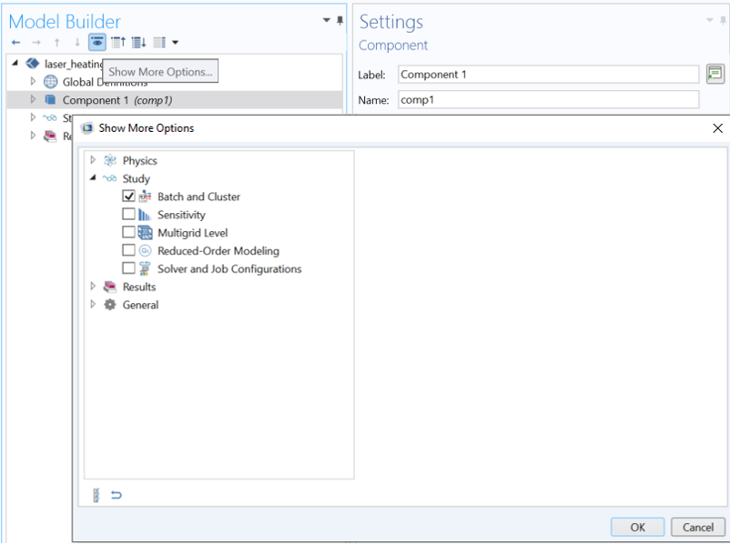
The Show More Options dialog box within the Model Builder.
Once this is enabled, you will be able to add a Batch Sweep feature to the Study branch. This feature will always exist at the very top of the Study, and can be thought of as a for-loop that wraps around all of the other study steps that exist beneath it within that Study branch.
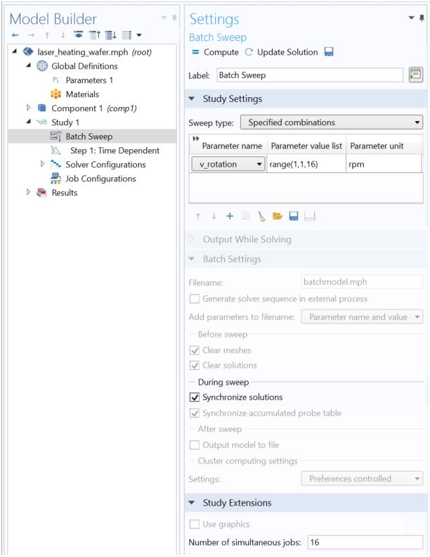
The relevant Batch Sweep feature settings.
The user interface for the Batch Sweep is shown above, with relevant features highlighted. First, at the very top, we specify the name of the parameter to sweep over and the number of different values of this parameter to study. Next, enabling the Synchronize solutions option will assemble all of the results back into a single file. If this is not enabled, then the batch sweep will just write a set of different files; one for each parameter in the sweep. (This may actually be an attractive option, as you can quickly get very large files, so it may also be worth considering if you want to save less data in each file.) The last key setting is at the bottom of the window: the number of simultaneous jobs, which determines how many jobs are run in parallel.
Also, keep in mind that the Batch Sweep can wrap around any other kind of sweep: Parametric, Function, Material, Auxiliary, or Frequency sweeps, so you can use a single Batch Sweep job to solve for an arbitrary combination of cases.
So, what number of jobs should we actually be running in parallel? That is the next question that we will look at.
How Much Batch Parallelism Can COMSOL Multiphysics® Exploit?
The answer to this question, as you’ve probably already surmised, is both hardware and model dependent.
In terms of model types, the ideal case for the Batch Sweep is a model that is small in terms of memory requirements, but takes a relatively long time to solve. A good example of such a model is the Laser Heating of a Silicon Wafer example. This model solves for the temperature evolution over time of a laser heat source moving over a rotating wafer. It has only about 2000 degrees of freedom, but takes about a minute of wall-clock time to solve on a typical desktop computer. There are a number of different parameters that we can sweep over in this model, so let’s see how this model’s performance scales with job parallelism on a typical modern desktop computer.
The results we will present were generated on an Intel® Xeon® W-2145 8-core processor with 32 GB RAM, a typical midrange computer as suggested in the COMSOL hardware recommendations. On this hardware, the test case model takes about one minute to solve. If we do a parametric sweep over 16 variations of the model, the solution time goes up about linearly with the number of different cases being solved. If we also use Batch Sweep, we can investigate running 2, 4, 8, and even 16 jobs in parallel on this hardware, with each batch sweep job containing a sequential parametric sweep, as shown in the screenshot below.
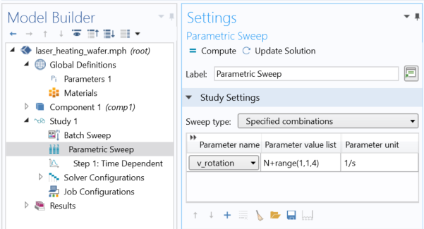
Screenshot showing a nested sweep. In this example, the outer Batch Sweep sweeps over N = 0,4,8,12, while the inner sweep results in 16 cases being solved in all.
The results below are presented in terms of time it takes to solve 16 cases and the relative speedup.
| Parametric Sweep | Batch Sweep + Parametric Sweep | ||||
|---|---|---|---|---|---|
| 16 sequential cases |
2 parallel jobs (8 sequential cases per job) |
4 jobs (4 cases/job) |
8 jobs (2 cases/job) |
16 jobs (1 case/job) |
|
| Time (Seconds) | 1010 | 620 | 416 | 305 | 267 |
| Speedup | 1 | 1.6x | 2.4x | 3.3x | 3.8x |
Observe from this data that as we run more jobs at the same time, we get more speedup. Most interestingly, we can see that we can solve 16 jobs in parallel on an 8-core machine and still observe speedup. In other words, each of the cores of this CPU can actually handle two COMSOL® jobs at once, at least when solving this particular model. Hyperthreading is enabled on this machine, and although that doesn’t speed up the solution itself, file opening and closing and other OS processes benefit from having hyperthreading enabled. Now, running so many cases in parallel does slow down the time that it takes to solve each single case, but the overall time taken for all 16 cases is less.
It’s also interesting to discuss what would happen if we tried to run more jobs in parallel, in terms of memory. This model needs about 1 GB of memory per batch job, and the test computer here has 32 GB RAM, so 16 parallel cases is no problem. But, if we went up to 32 parallel cases, we could exceed the available RAM, which would lead to a slowdown, regardless of the number of cores. Of course, on a computer with more RAM, more cores, and multiple CPUs, we can get even more relative speedup. Furthermore, COMSOL Multiphysics does not limit the number of cores, or CPUs, that can be addressed on a single computer.
Now, these data look quite nice, and you are almost certainly tempted to ask at this point if you will always get results this good. Unfortunately, the answer is: not always. The larger the model that we solve, the less speedup we will see. For very large models, there will be an overall slowdown if you run jobs in parallel. However, for a great many models, especially most 2D models and smaller 3D models, you can reasonably expect similar improvement when using Batch Sweep on multicore, multi-CPU computers. So, the Batch Sweep functionality can strongly motivate investing in such hardware. Also, there is a lot of other power to the Batch Sweep functionality that is discussed in this previous blog post. Keep in mind that this is a core capability of COMSOL Multiphysics available with all license types!
Intel and Xeon are trademarks of Intel Corporation or its subsidiaries.

Comments (2)
Helger van Halewijn
February 6, 2023Preparing a batch job in a similar way as posted in the blog.
It is not clear to me why you use this setup.
I would like to use the parameter of simultaneous jobs as a parameter in the : Number of simulteneous jobs. For example that one automates the whole sequence by scanning the time durations as a function of the parallel jobs.
Could you comment on this?
Regards,
Helger.
Walter Frei
February 6, 2023 COMSOL EmployeeThe “Number of simultaneous jobs” can only be a scalar, not a parameter that you sweep over. That kind of investigation has to be done one set at a time, manually. It should be emphasized that there likely is no generalization that one can make about an optimum number for this setting, it is entirely problem, problem size, and hardware dependent. See also: https://www.comsol.com/blogs/much-memory-needed-solve-large-comsol-models/