

When a drop of water gets attached to a metallic surface, general corrosion may be initiated. In some cases, and if there is enough contact time, a very small pit may be formed at the metallic surface due to this corrosion. The conditions in such a pit may develop over time so that the bottom of the pit becomes a net anodically polarized surface, while the area away from the mouth of the pit acts as a net cathodic surface. This accelerates the corrosion at the bottom of the pit and a large pit may be formed. Modeling pitting corrosion serves the purpose of understanding how a certain material or a certain design may be susceptible to pitting corrosion under certain conditions. This blog post shows what a model for studying pitting corrosion may look like.
Introduction to Corrosion Processes
Galvanic corrosion is driven by the electronic and ionic contact of two metals with different affinities to electrons. If two such metals are put in contact with the same electrolyte, they form charged double layers at their surface against the electrolyte. The voltage over this charged double layer is different for the two metals. This results in electrons being conducted from the less noble metal to the more noble metal, as shown in Figure 1.
At the noble metal surface, these electrons may take part in a charge transfer reaction, which, at the noble metal, is a net reduction reaction (cathodic reaction). At the less noble metals, electrons are taken, and this charge transfer reaction may result in the dissolution of the less noble metal in a net anodic reaction.
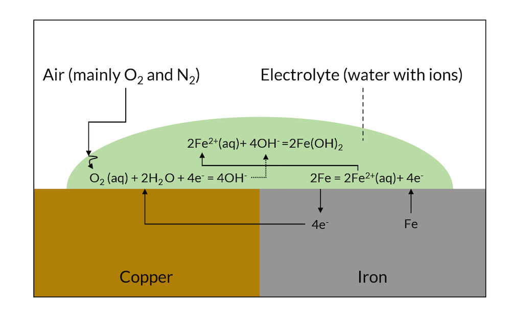
Figure 1. Schematic description of galvanic corrosion.
When the reactions in Figure 1 have been allowed to proceed for a while, then the less noble metal (iron in this case) may have dissolved close to the contact surface to the more noble metal, as shown in Figure 2 below.
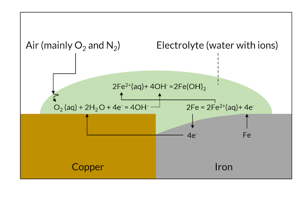
Figure 2. After a while, galvanic corrosion may have dissolved part of the iron metal close to the copper contact area.
We can now look at a drop of water on the surface of a single metal; see Figure 3. The microscopic structure may have regions with different metal phases, which may have slightly different electron affinities. This means, for example, that cathodic reactions may occur in metal crystallites, while anodic reactions may occur in the intergranular areas.
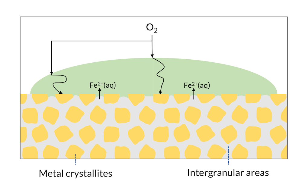
Figure 3. Areas of a metal surface may consist of crystals and intergranular areas.
In Figure 2, iron hydroxide may be formed close to the surface where iron is released. This is one of the components in rust. In Figure 3, the formation of rust may occur all over the surface, since the intergranular areas are so evenly distributed. This is usually referred to as generalized corrosion.
Let us now look at Figure 4, where the process in Figure 3 has been allowed to continue. The transport of oxygen to the crystallite surface is longer in the middle of the drop compared to the edges, where the oxygen diffusion length is smaller. The metal surface in the middle of the drop is depleted of oxygen, which lowers the potential of this region compared to the areas in the edges of the drop. This lowers the potential below the passivation potential for iron, which may destabilize the iron oxide protective layer. Eventually, the crystallites in the middle of the surface may act as net anodes, due to oxygen depletion. This leads to the initialization of a pit through iron dissolution in the middle of the drop. The production of iron ions also yields a reaction with water, where protons are formed, thus lowering pH in the pit. The lowered pH results in an even more accelerated corrosion rate. This process is referred to as the Evans drop experiment (Ref. 1) after the scientist who first explained and reproduced this process.
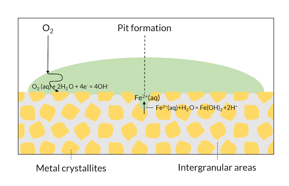
Figure 4. The Evans drop experiment. The formation of a pit also leads to a lowered pH in the pit, which accelerates the anodic reaction even more.
The initialization of a pit may occur with other mechanisms. For example, mechanical indentations or impurities in the metal surface may weaken the oxides that partially protect the iron surface from further corrosion. Stainless steel especially has a protective oxide layer that may be damaged mechanically or chemically.
Modeling Pitting Corrosion
The model in this blog post starts with the pit already formed. We also assume that we have a very large area outside of the modeled domain, which gives a stable mixed potential that is not affected by the local current to any larger extent. This also gives a constant electrolyte potential away from the pit.
The reactions that are accounted for are:
- Iron dissolution at the anodically polarized surfaces: \[2Fe = 2F{e^{2 + }}\left( {aq} \right) + 4{e^ – }\]
- Precipitation reaction in the electrolyte: \[F{e^{2 + }}\left( {aq} \right) + 2O{H^ – } = Fe{\left( {OH} \right)_2}\left( s \right)\]
- Water autoprotolysis in the electrolyte: \[{H_2}O = {H^ + } + O{H^ – }\]
The modeled chemical species are the following:
- \[F{e^{2 + }}\]
- \[{H^ + }\]
- \[O{H^ – }\]
- \[N{a^ + }\]
- \[C{l^ – }\]
The concentration of hydroxyl ions can be eliminated by assuming that the water autoprotolysis is at equilibrium. One of the other ions, in this case the proton, can be eliminated using the electroneutrality condition. Both of these eliminations are automatically taken care of in the COMSOL Multiphysics® software by the Tertiary Current Distribution, Nernst-Planck interface by selecting the Water-based with electroneutrality option. Note though that the transport equations for all of the ions are included in the balance of current in the expression for the electrolyte current density. The last dependent variable is the electrolyte potential.
For the initial state, we assume that the precipitation reaction has created a deposit inside of the pit so that the pit can be considered a porous structure, where the electrolyte fills the pores. This is a reasonable assumption, since the deposits may very well be formed from the metal that used to be in the location where the pit is. Furthermore, the model domain is assumed axisymmetric, as shown in Figure 5.
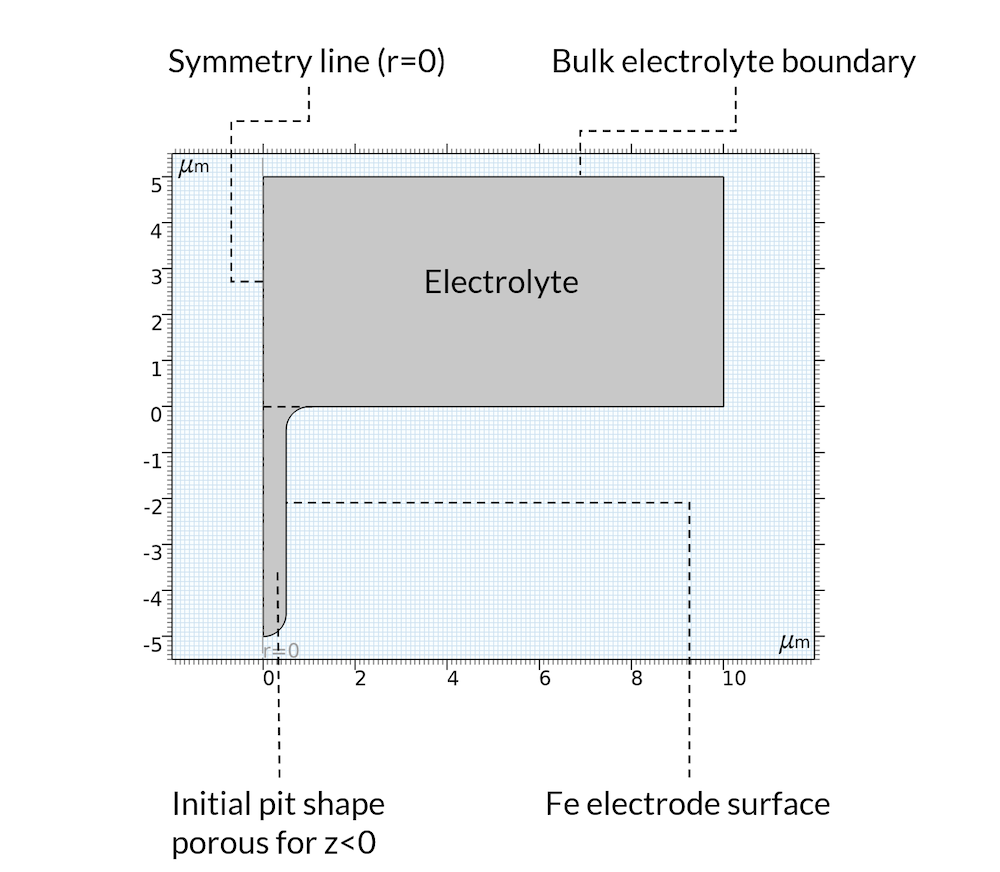
Figure 5. Geometry and boundaries of the model domain.
The metal dissolution reaction is defined all over the boundary denoted “Fe electrode surface” in Figure 5 above. The anodic reaction rate is assumed proportional to the proton concentration. This is valid for acidic conditions in the presence of chloride (Ref. 2). The iron dissolution reaction is coupled to the displacement of the boundary using moving mesh.
As mentioned above, we do not model the oxygen reduction reaction. Instead, we set a constant electrolyte potential far away from the pit at a horizontal position, which we have denoted “Bulk electrolyte boundary”. At this boundary, we also set the sodium, chloride, and iron ion concentration.
In the electrolyte domain, including the pit, we assume that both the water autoprotolysis and the iron hydroxide reactions occur. Note that as hydroxide is consumed through the production of Fe(OH)2 (s), this also drives the lowering of pH, which was previously mentioned in Figure 4.
The initial concentration of species and the initial electrolyte potential is computed by solving the problem for the initial geometry assuming that the process is in quasi steady state. This means that the problem is solved for a fixed geometry, with the boundary conditions mentioned above, using a stationary solver. This results in a certain composition profile and electrolyte potential distribution already at t = 0. This solution is the initial condition for the time-dependent study.
Results
The initial quasi steady state seems to be a reasonable assumption, since the change in electrolyte composition and potential is relatively slow in the beginning, between 0 and 1 day.
Figure 6 below shows the growth of the pit over 30 days. The gradient of the electrolyte potential is large inside the pit. The electrolyte potential varies between 0.43 mV and 16.5 mv in the pit, while it varies from 0 mV to 0.43 mV outside of the pit after 30 days. Note that the transport is slower in the pit, since we assume a porous media with lower effective transport properties compared to the electrolyte outside. The same qualitative potential distribution is observed over the whole modeled period of time with the observation that the pit’s bottom grows faster than the pit’s mouth. This results in a relatively narrower path for the current at the pit’s mouth, resulting in larger gradients in the electrolyte potential at the mouth. Note that we do get some corrosion at the flat surface. Over 30 days, the displacement of the surface is about 0.35 μm, while the same displacement for the bottom of the pit is 1.45 μm.

Figure 6. The bottom of the pit grows faster than the mouth of the pit. This leads to a larger gradient in the electrolyte potential close to the mouth.
The change in pH during the corrosion process is shown in Figure 7 below. The pH at the bottom of the pit after 1 day is 9.48, and it is 9.14 after 30 days. This may not seem like a large change, but it corresponds to a factor of 2.2 higher proton concentration after 30 days compared to after 1 day. The rate constant for the corrosion process is proportional to the proton concentration, which also means that the corrosion rate is accelerated correspondingly.

Figure 7. The pH in the pit at different times.
Figure 8 shows the corrosion rate in μm/day for the four times plotted above. The maximum corrosion rate at the bottom of the pit is 2.3 higher after 30 days compared to the corrosion rate after 1 day. This is in line with the proton concentration being 2.2 higher after 30 days compared to 1 day.

Figure 8. Corrosion rate at the metal surface at different times.
The concentration profile of sodium ions is the opposite of the profile for the iron ions. The reason is the electroneutrality condition. As iron ions are pushed into the electrolyte, the sodium ions are pushed out of the pit. Contrary to the sodium ions, the chloride ions are pushed into the pit in order to preserve electroneutrality (not shown).

Figure 9. The sodium ion concentration at different times.
The model clearly shows the “vicious circle” aspect of pitting corrosion. The process accelerates with time until the pit is deep enough so that the ohmic losses and corrosion products become limiting.
Concluding Remarks
A simple possible extension to this model is to account for the material balance of the precipitated corrosion products. These products have a lower density than the iron metal, so they will form in the pit but will also be pushed outside of the pit. This could be modeled by introducing porosity as a dependent variable with transport given by the advection of the oxides.
Another natural extension of the model is to account for the full drop geometry in order to include oxygen diffusion and oxygen reduction.
The third extension to the model would be to include more detailed chemistry, for example, by including more iron ions, more possible redox reactions, as well as more iron oxides and hydroxides at the surface of the metal. Meanwhile, we can play with the existing model, which is quite advanced despite the relatively simple modeling procedure.
Next Steps
- Learn more about the specialized features and functionality in the Corrosion Module
- Try modeling pitting corrosion yourself by downloading this related tutorial model
References
- U.R. Evans, “Corrosion and Oxidation of Metals”, Amolds, p. 118., 1960.
- H.C. Kuo and K. Nobe, “Electrodissolution Kinetics of Iron in Chloride Solutions”, J. of Electrochem. Soc, vol. 125, no.6, 1978.


Comments (18)
jean michel Puybouffat
July 20, 2021brillant paper
i need to understand how works multipysics . what is the way to use what we need to work with
M. Rashed Khan
March 25, 2022Ed, do you have the model files? Can I have a copy of the model file to learn more?
Ed Fontes
March 28, 2022 COMSOL EmployeeDear Rashed,
Here it is:
——————————————-
http://cds.comsol.com/mg/1624145ee543a8.zip
Estimated size: 9.0 MB
This link expires April 4, 2022. Please make sure to download before that date.
Included files:
– pitting_corrosion.mph
——————————————-
Best regards,
Ed
Тимур Николаевич Терентьев
May 12, 2022Dear Ed,
Unfortunately the link is out of date.
Can I have a copy of the model file too?
Best regards,
Tim
Ed Fontes
August 29, 2022 COMSOL EmployeeHi Tim,
Here is a new link:
——————————————-
https://cds.comsol.com/mg/f630c73e81e7e5.zip
Estimated size: 9.0 MB
This link expires September 5, 2022. Please make sure to download before that date.
Included files:
– pitting_corrosion.mph
——————————————-
Best regards,
Ed
Mason Chen
August 26, 2022Hi Ed,
Could you please upload the link for the model again? I am interested in it. Thank you very much.
Ed Fontes
August 29, 2022 COMSOL EmployeeHi Mason,
Heres is a new link:
——————————————-
https://cds.comsol.com/mg/f630c73e81e7e5.zip
Estimated size: 9.0 MB
This link expires September 5, 2022. Please make sure to download before that date.
Included files:
– pitting_corrosion.mph
——————————————-
Best regards,
Ed
Zine Eddine Kribes
September 20, 2022Hi Ed,
Could you please upload the link for the model again? I am interested in it. Thank you very much.
Zine.
Hossein Moradi
February 20, 2023Dear Ed,
Can I select more than 5 species for a time-dependent study with geometry deformation?
Ed Fontes
February 20, 2023 COMSOL EmployeeDear Hossein,
Yes, you can add more than 5 species. You can add an arbitrary number of species until your CPU and RAM becomes limiting.
Best regards,
Ed
Cemal Ozturk
March 6, 2023Hi Ed, could you please upload again? Have a great week and stay safe!
Ed Fontes
March 9, 2023 COMSOL EmployeeHi Cemal,
The model is now available for download in the Application Gallery:
https://www.comsol.com/model/pitting-corrosion-100101
Stay safe you too!
Best regards,
Ed
Yassine El Kouri
March 15, 2023Hello Ed, I’ve just gotten access to the simulation file and I wish to run a pitting corrosion of an Aluminum alloy using this file, what are the changes that I have to make ? Cheers
Hossein Moradi
March 20, 2023Dear Ed;
Will this model converge for more time, for example for 60 days?
Giancarlo Consolo
March 20, 2023Dear Ed,
I’ve a very similar question to the one raised by Hossein.
I’ve noticed that simulation does not converge for time larger than 45 days due to the generation of an inverted element of the mesh.
Any suggestion on how to extend the simulation time? Just refinining the mesh?
Many thanks in advance
Jiejie Wu
August 14, 2023Hi Ed, very useful article, thanks!
For your second recommended extension of the model (to account for the full drop geometry in order to include oxygen diffusion and oxygen reduction), the pit size is very small (1um diameter), but the drop could be a few mm or even 1cm. Do you have recommendations how to model the full geometry? How would you set the boundary conditions for the edge of the drop, and the electrolyte initial potential?
Thanks,
Jiejie
Ed Fontes
August 17, 2023 COMSOL EmployeeDear Jiejie,
Thank you for your kind words.
You have a good point. I was actually thinking about brute force here. For a mm-size droplet, then that would be a model of around 10 MDOF, which should not be a problem (100 MDOF is also OK on a cluster).
Another possible but maybe far-fetched approach would be to couple a finite element (FEM) and a boundary element method (BEM), using FEM close to the pit and BEM for the rest of the droplet. But then you can only use BEM in a decoupled way, since the method does not support nonlinear problems. This sounds more difficult and I have never really considered this method for this problem.
I will have to try both approaches (brute force and FEM-BEM)…
Best regards,
Ed
Jiejie Wu
August 17, 2023Hi Ed,
Sounds promising! I wonder how many cores would be required to handle 10 MDOF? We have some computing cluster, but not sure if enough.
It would be great to hear about how you doing with your two approaches after you try. I look forward to that.
Kind regards,
Jiejie