Ray Optics Module Updates
For users of the Ray Optics Module, COMSOL Multiphysics® version 5.5 brings multiscale modeling with new features to couple frequency-domain electromagnetics with the RF Module or Wave Optics Module to ray optics, a dedicated Spot Diagram plot that makes postprocessing much easier, and improvements to the Grating boundary condition, including a dedicated Cross Grating feature. Learn about these and other Ray Optics Module updates in more detail below.
Multiscale Electromagnetics Modeling
Two new ray release features enable multiscale electromagnetics modeling with the Ray Optics Module in combination with the RF Module or the Wave Optics Module. The functionality is seamless and fully integrated in the Model Builder workflow.
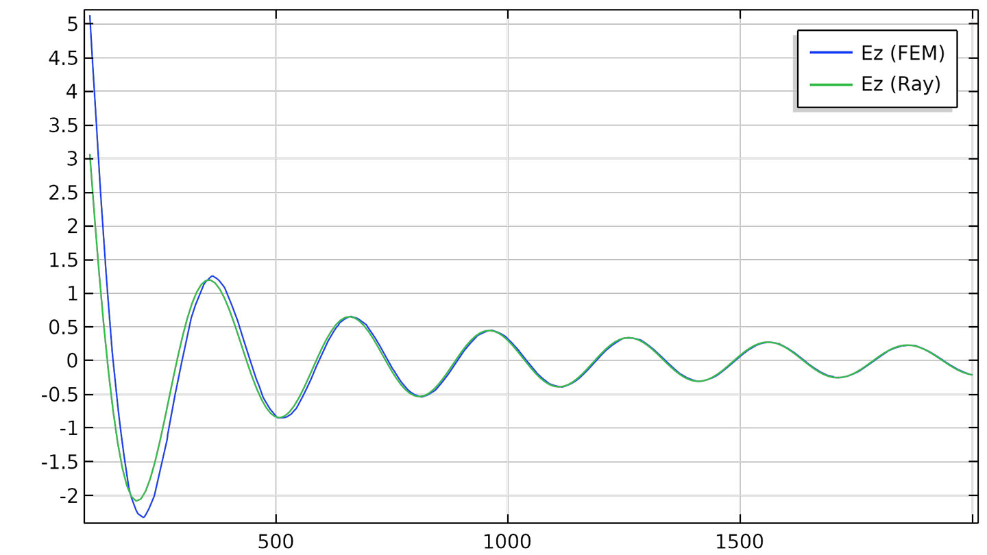
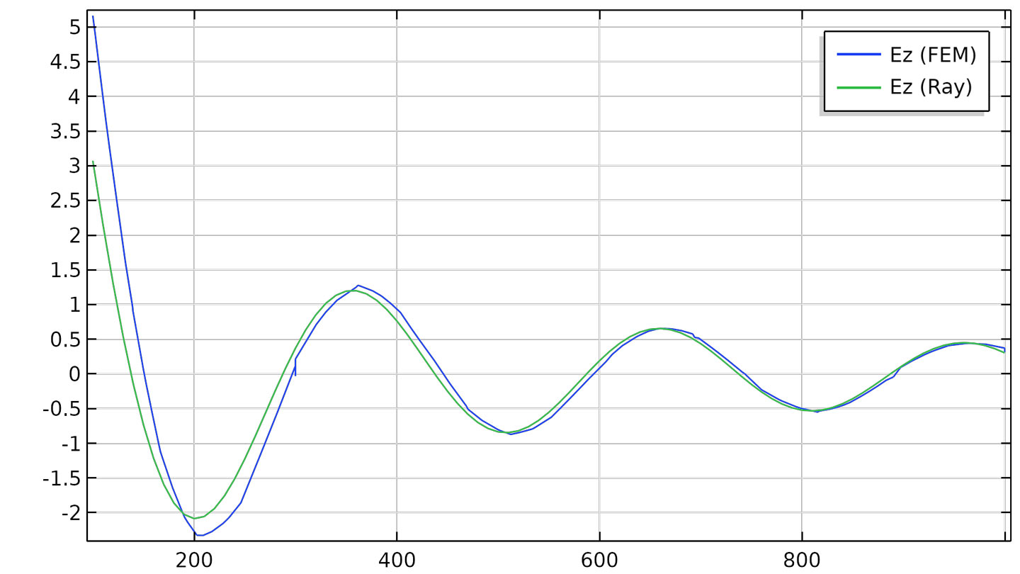
In this case, multiscale means that waves are modeled over length scales comparable to the wavelength as well as length scales that could be much larger. The finite element method (FEM) is used at the wavelength scale and a ray tracing approach is used for modeling propagation over long distances.
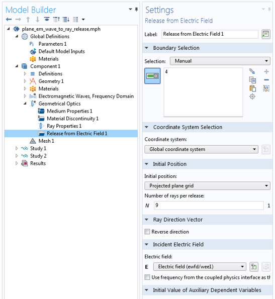
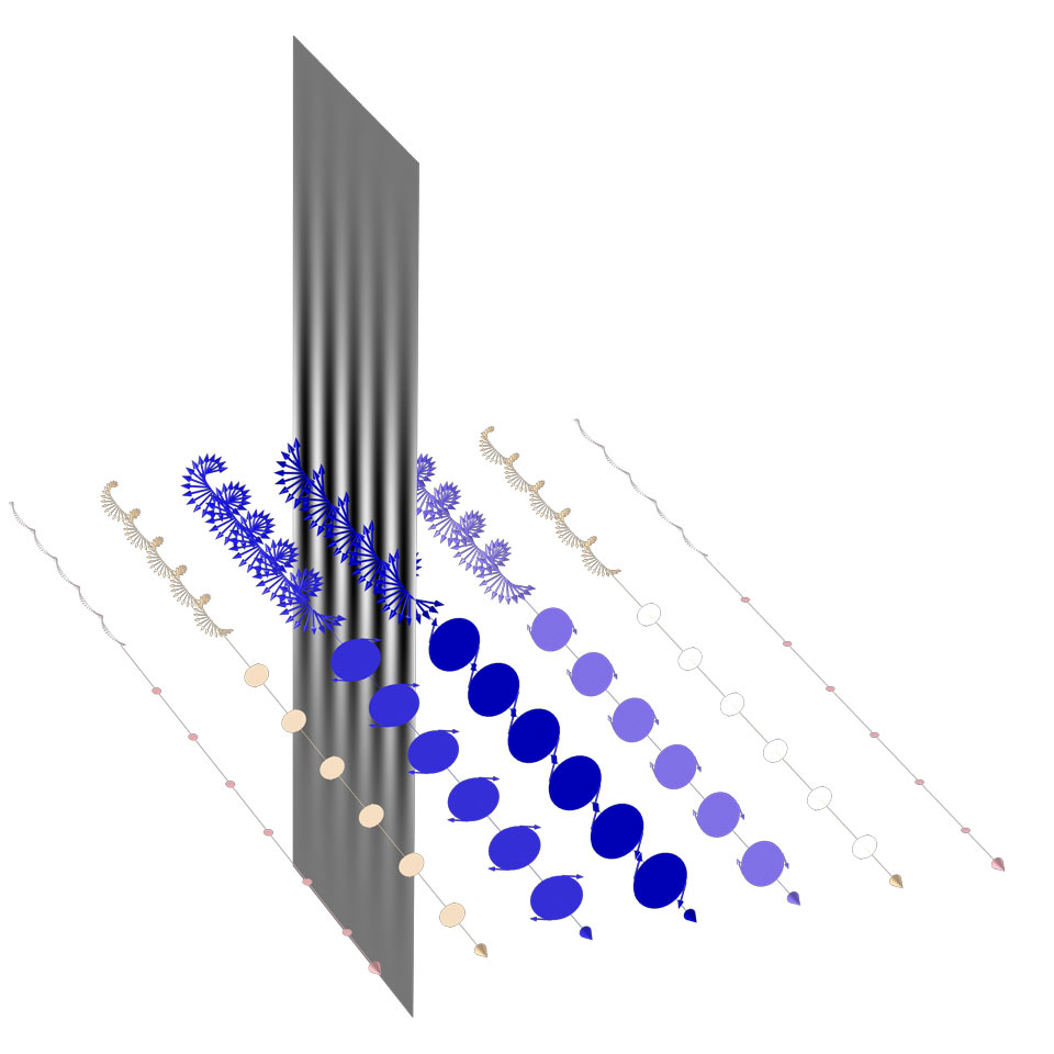
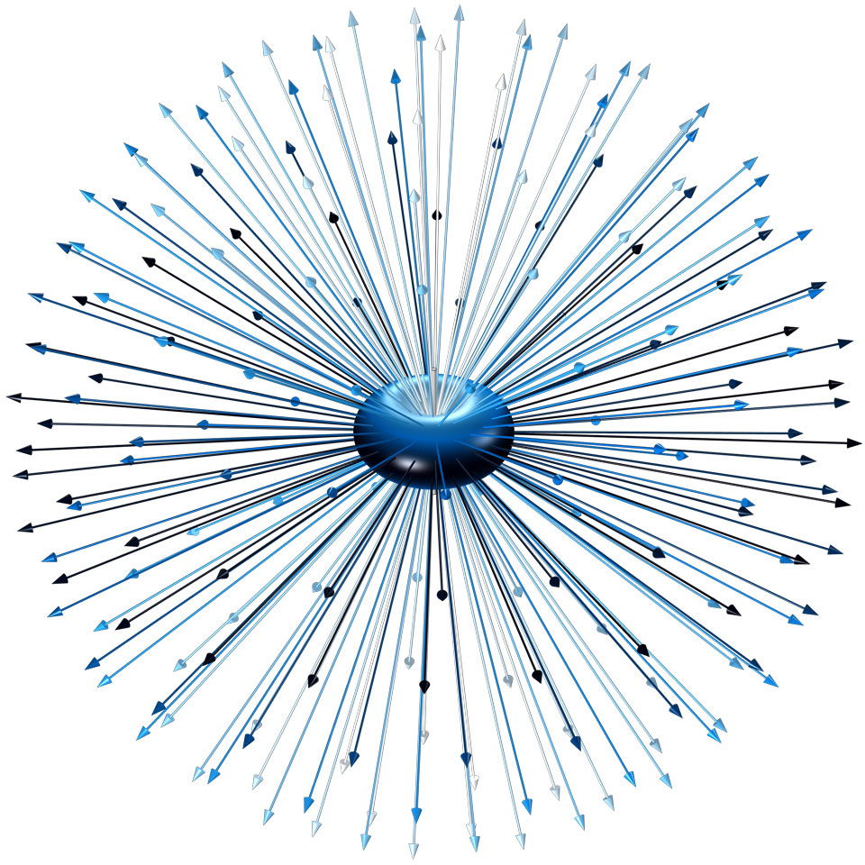
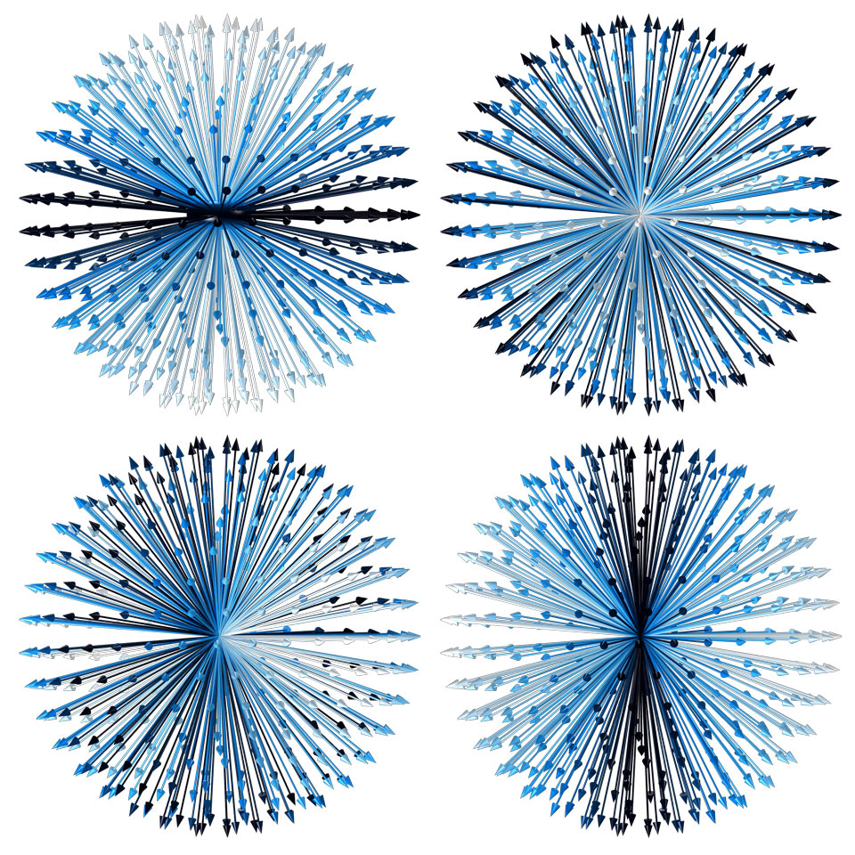
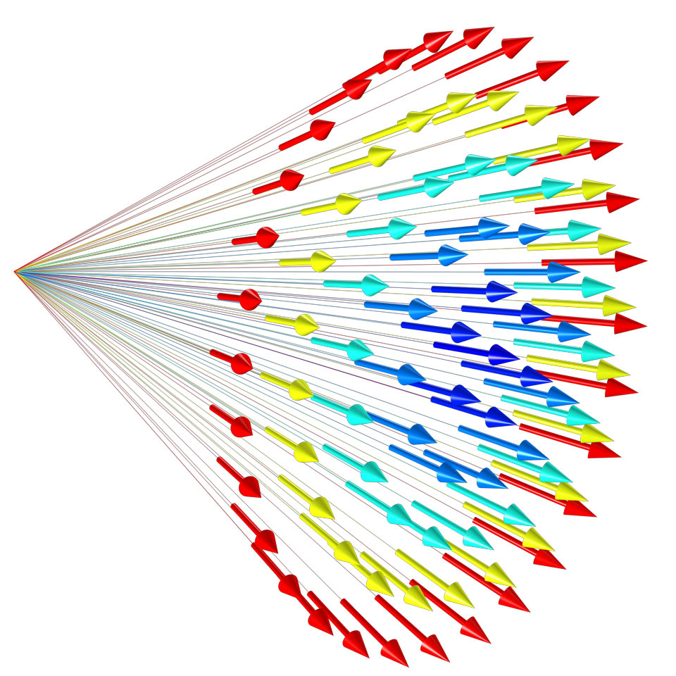
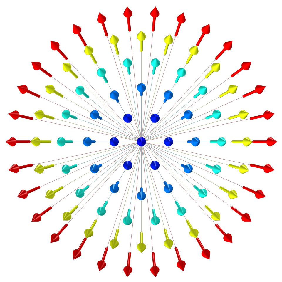
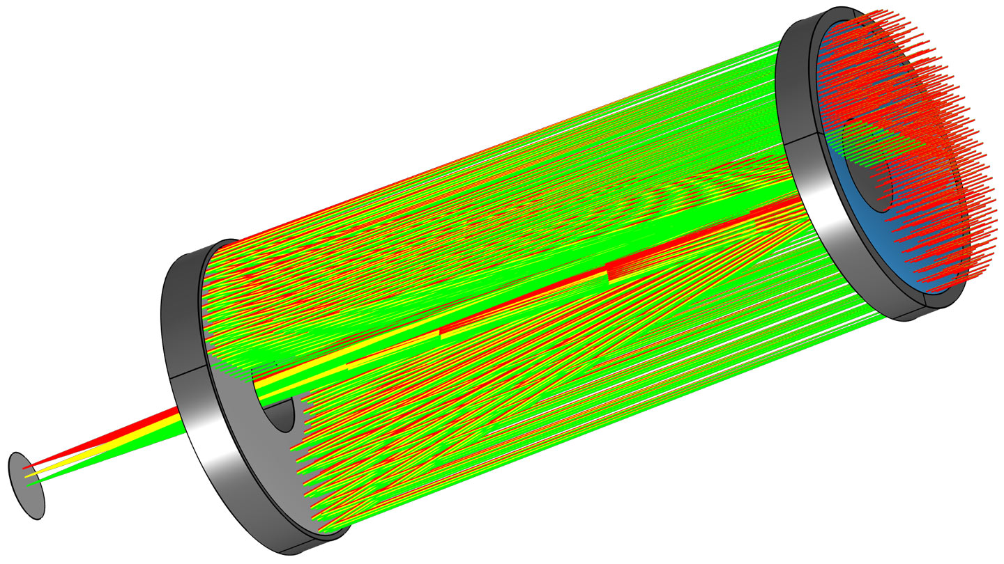
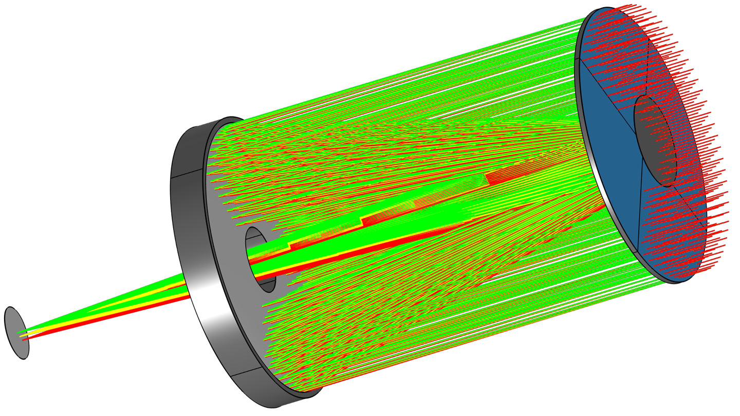
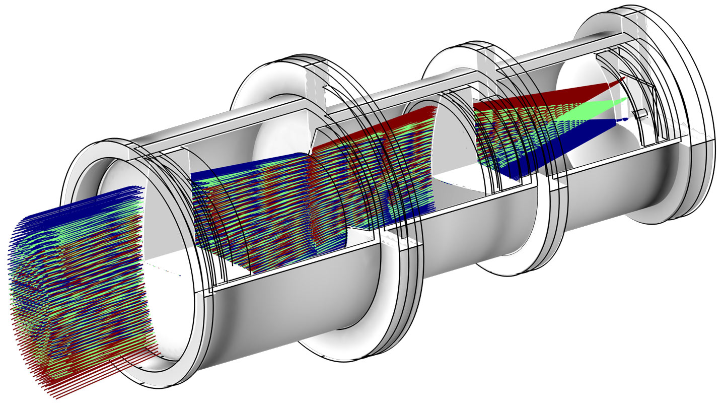
Use the new Release from Electric Field feature to launch rays from a surface; the initial intensity and polarization of the rays are taken from the electric field in an adjacent region. This allows you to first model electromagnetic wave propagation over a distance comparable to the wavelength, using the Electromagnetic Waves, Frequency Domain interface or Electromagnetic Waves, Beam Envelopes interface, and then extend the model over a much longer distance via ray tracing. Similarly, you can use the new Release from Far-Field Radiation Pattern feature to launch rays outward from a point, or grid of points, based on a far-field function defined in a previous study. When releasing rays, you can transform the radiation pattern by specifying Euler angles. This allows you to release rays from many different antenna orientations, without having to recompute the radiation pattern.
You can see this new functionality in the following models:
- plane_em_wave_to_ray_release (New model)
- ray_release_from_dipole_antenna_source_2daxi (New model)
- ray_release_from_dipole_antenna_source_3d (New model)
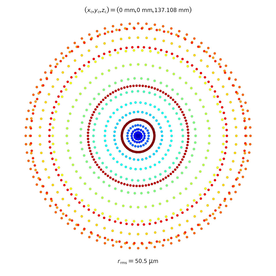
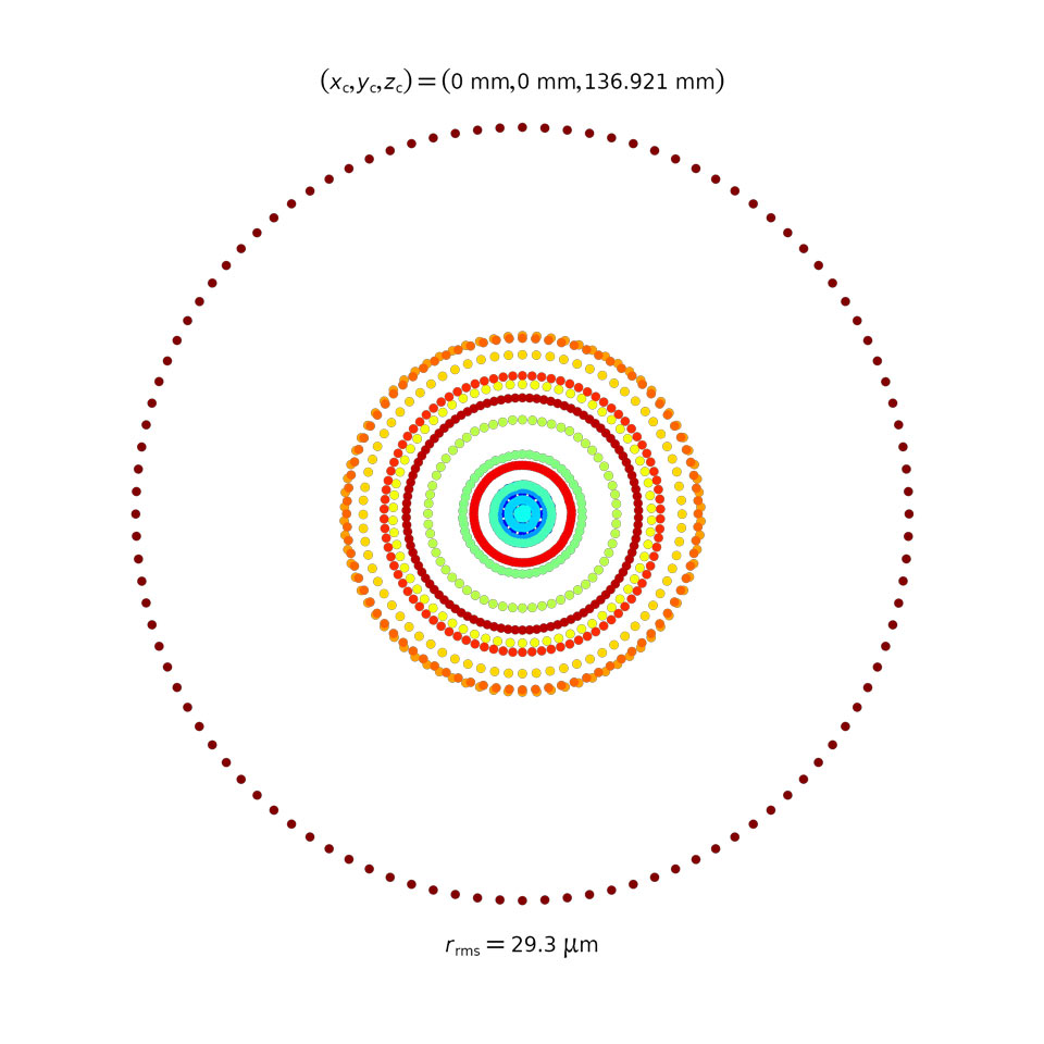
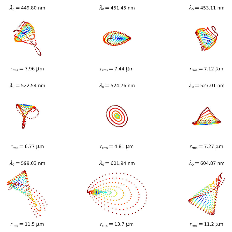
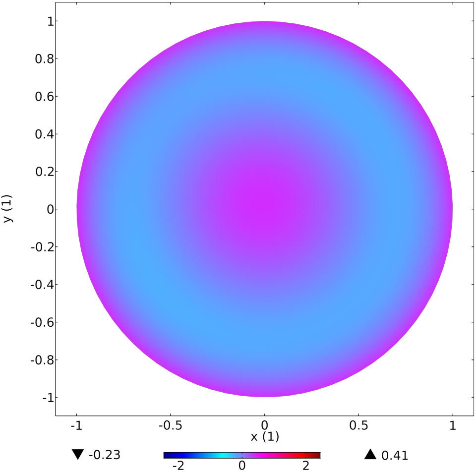
Spot Diagram Plot
With the dedicated Spot Diagram plot, you can more easily plot the intersection points of rays with a surface, significantly speeding up the postprocessing of ray optics models. The surface can either be a physical boundary in the geometry or a virtual boundary created by the Intersection Point 3D dataset.
The Spot Diagram plot includes dedicated tools for customizing and organizing the plot, such as:
- Filtering rays out so they do not appear in the plot
- Sorting the rays based on wavelength or field angle so they appear as an array of distinct spots
- Automatically locating the plane of minimal root mean square (RMS) spot size and creating a dataset there
- Displaying text annotations such as spot size, wavelength, and position
You can see this new functionality in the following models:
- compact_camera_module (new model)
- cross_grating_echelle_spectrograph (new model)
- double_gauss_lens
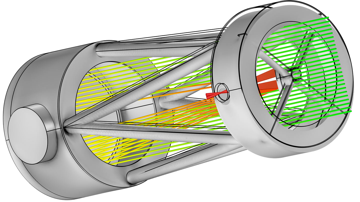
- gregory_maksutov_telescope (new model)
- hubble_space_telescope
- keck_telescope (new model)
- luneburg_lens_go
- newtonian_telescope
- newtonian_telescope_structural_analysis (new model)
- petzval_lens
- petzval_lens_stop_analysis (new model)
- petzval_lens_stop_analysis_isothermal_sweep (new model)
- petzval_lens_stop_analysis_with_hyperelasticity (new model)
- petzval_lens_stop_analysis_with_surface_to_surface_radiation (new model)
- schmidt_cassegrain_telescope (new model)
- thermally_induced_focal_shift
- white_pupil_echelle_spectrograph
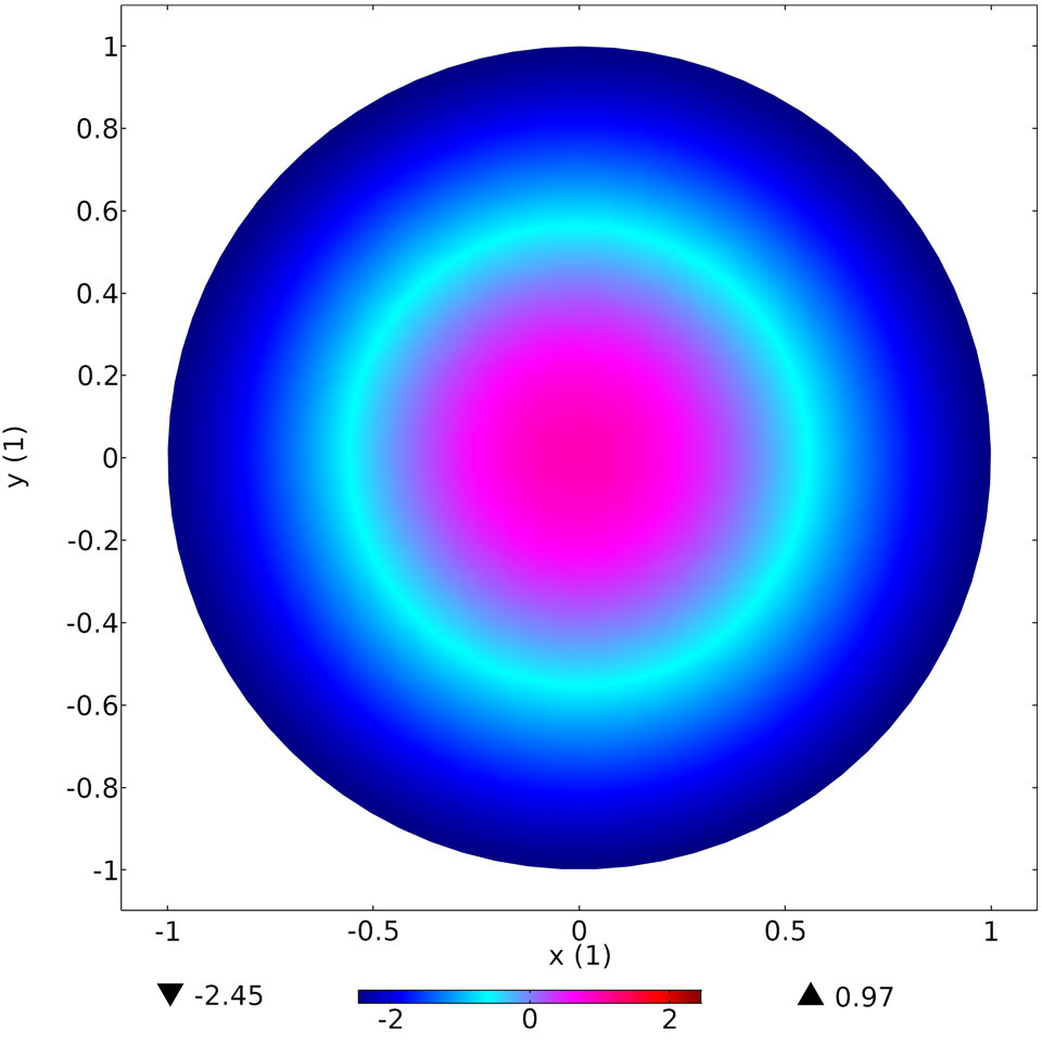
Improvements to the Optical Aberration Plot
The Optical Aberration plot has new settings that make it easier to compute the Zernike polynomial coefficients that describe monochromatic aberrations. There are built-in filter options to remove rays based on wavelength, number of reflections, or release feature. There is also a new command to automatically define a reference hemisphere centered at the rms focus. You can see this new functionality in the Double Gauss Lens and Newtonian Telescope Structural Analysis models.
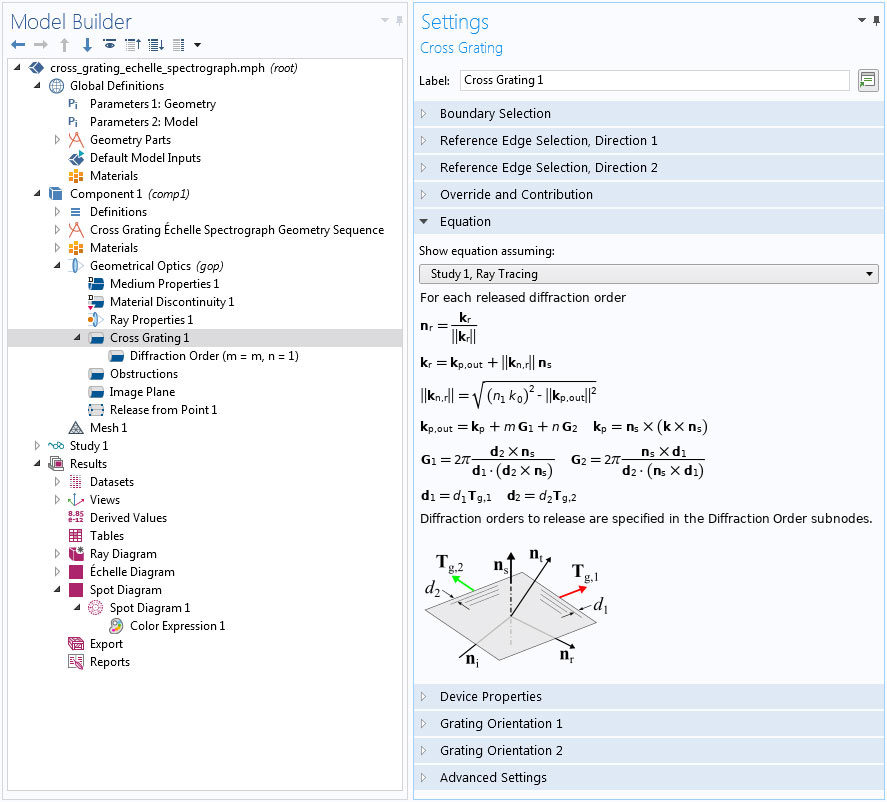
Cross Grating Feature
Use the new Cross Grating feature to treat a boundary as a periodic substructure with two different directions of periodicity. In contrast, the existing Grating node allows one direction of periodicity and treats the substructure as homogeneous in the orthogonal direction. You can see this new functionality in the Cross Grating Échelle Spectrograph model.
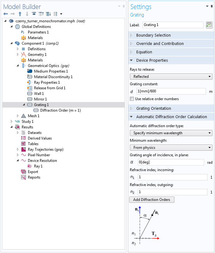
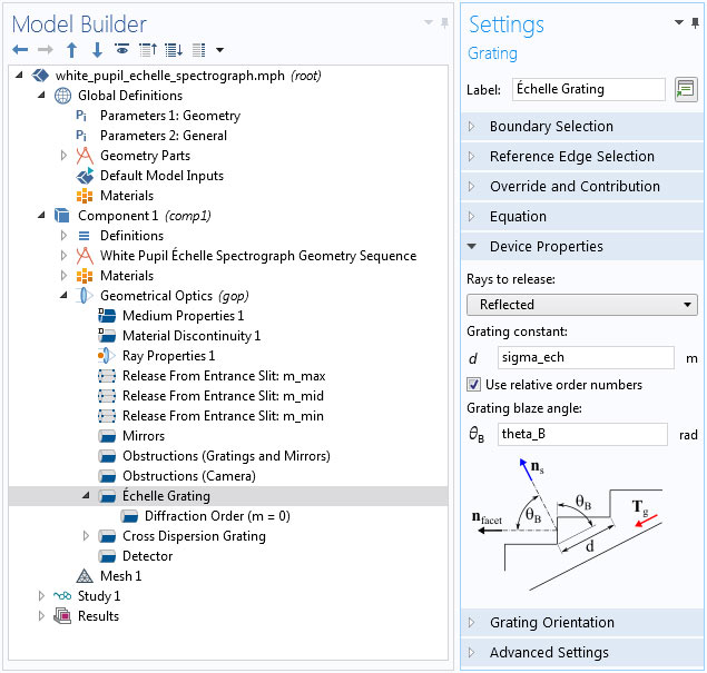
Grating Improvements
The Grating feature has been significantly upgraded in version 5.5. You can now click an Add Diffraction Orders button to automatically create subnodes for all of the diffraction orders that the grating might release, based on the wavelengths of rays used in the model. Alternatively, you can specify relative diffraction orders for the grating. This is particularly useful in blazed gratings, where the absolute diffraction orders with the lowest relative order numbers are those that show the smallest deviation from the blaze angle. You can see this new functionality in the White Pupil Échelle Spectrograph model.
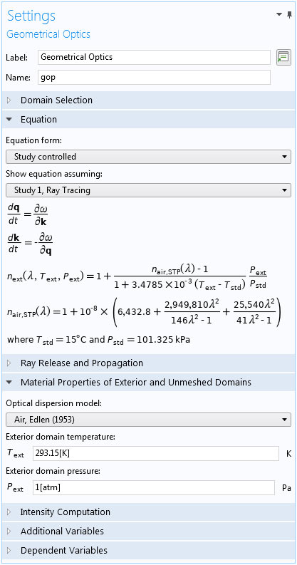
Air Model for Exterior and Void Domains
You can now treat the empty space outside the geometry, and in unmeshed domains, as air using the built-in Edlen model, which accurately expresses the refractive index of air as a function of temperature and pressure. This allows you to easily model optical systems that have been optimized for atmospheric, rather than vacuum, conditions. As always, exterior and unmeshed domains must be homogeneous. The exterior temperature and pressure are scalar inputs that must apply over the entire region.
You can see this new functionality in the following models:
- compact_camera_module (new model)
- cross_grating_echelle_spectrograph (new model)
- double_gauss_lens
- petzval_lens
- petzval_lens_stop_analysis (new model)
- petzval_lens_stop_analysis_isothermal_sweep (new model)
- petzval_lens_stop_analysis_with_hyperelasticity (new model)
New Release Type: Hexapolar Cone
When you release rays in a cone, a new type of Conical distribution is available: Hexapolar. For the Hexapolar cone option, rays are released at uniformly distributed angles from the cone axis, with each ring having six more rays than the previous one.
You can see this new functionality in the following models:
- cross_grating_echelle_spectrograph (new model)
- thermally_induced_focal_shift
- white_pupil_echelle_spectrograph
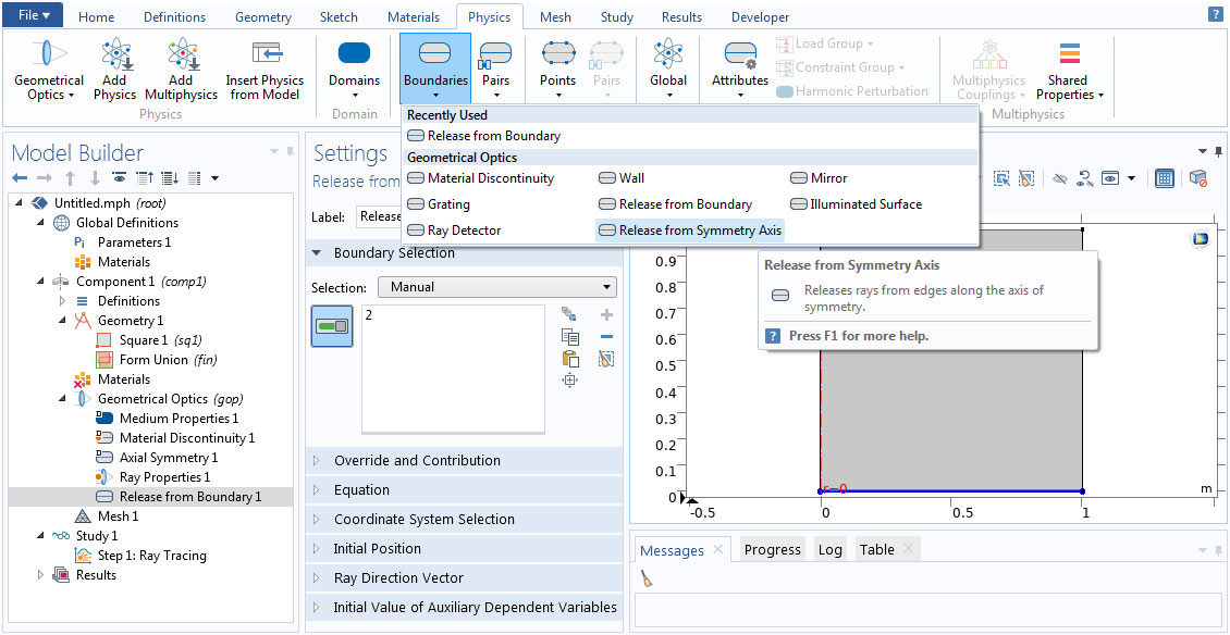
Renamed Ray Release Features
Ray release features have been renamed in COMSOL Multiphysics® version 5.5. The Inlet is now called Release from Boundary, and the Inlet on Axis (in 2D axisymmetric models) is now called Release from Symmetry Axis.
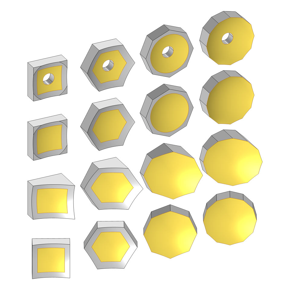
New Polygonal Mirror Parts
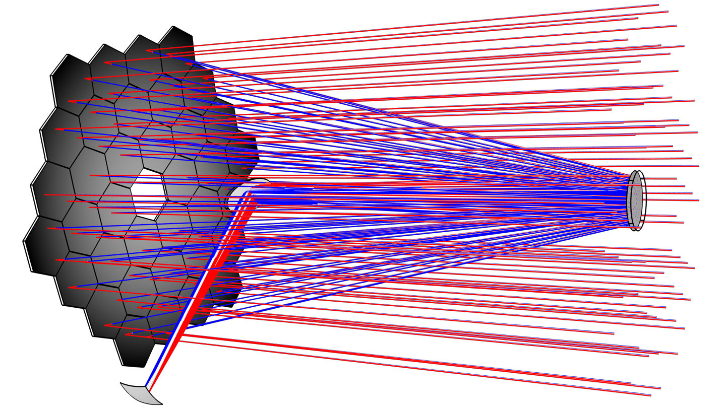
You can now add polygonal mirrors to the geometry using the Part Libraries for the Ray Optics Module. The new polygonal mirrors are named Spherical Polygonal Mirror 3D, Conic Polygonal Mirror On Axis 3D, and Conic Polygonal Mirror Off Axis 3D. You can see the Conic Polygonal Mirror Off Axis 3D part used in the Keck Telescope model.
Aspheric Lens and Mirror Parts
The aspheric lenses and mirrors in the Part Libraries for the Ray Optics Module have been revised, and several new parts are available:
- Aspheric Even Lens 3D (improved replacement for the Aspheric Lens 3D, which has moved to legacy parts)
- Aspheric Even Mirror 3D
- Aspheric Odd Lens 3D
- Aspheric Odd Mirror 3D
- Aspheric Q-type Qbfs Lens 3D
- Aspheric Q-type Qbfs Mirror 3D
- Aspheric Q-type Qcon Lens 3D
- Aspheric Q-type Qcon Mirror 3D
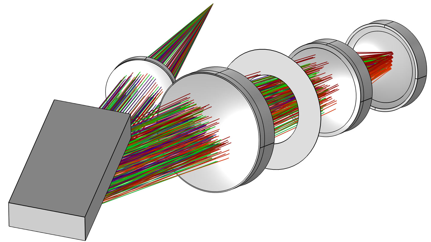
Here, "Q-type" indicates a type of orthogonal polynomial basis that is used to define the lens or mirror surface sag. "Qbfs" and "Qcon" indicate that the polynomials describe the deviation from a "best-fit sphere" and a conic, respectively. The advantage of defining Q-type aspheres over the even and odd aspheres is that all of the polynomial coefficients have about the same order of magnitude, so there is less risk of numerical error due to roundoff. You can see the Aspheric Even Lens 3D used in the Compact Camera Module and Schmidt Cassegrain Telescope models.
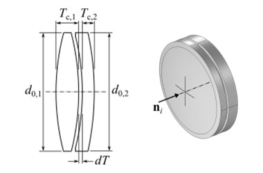
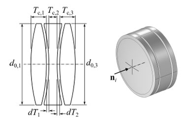
Doublet and Triplet Lens Parts
Two new multiplet lens parts are now available in the Part Libraries for the Ray Optics Module: Spherical Doublet Lens 3D and Spherical Triplet Lens 3D. For both of these parts, you can specify whether the individual lenses are cemented together or if there is an air gap between them. You can see the Spherical Doublet Lens 3D in the Cross Grating Échelle Spectrograph model.
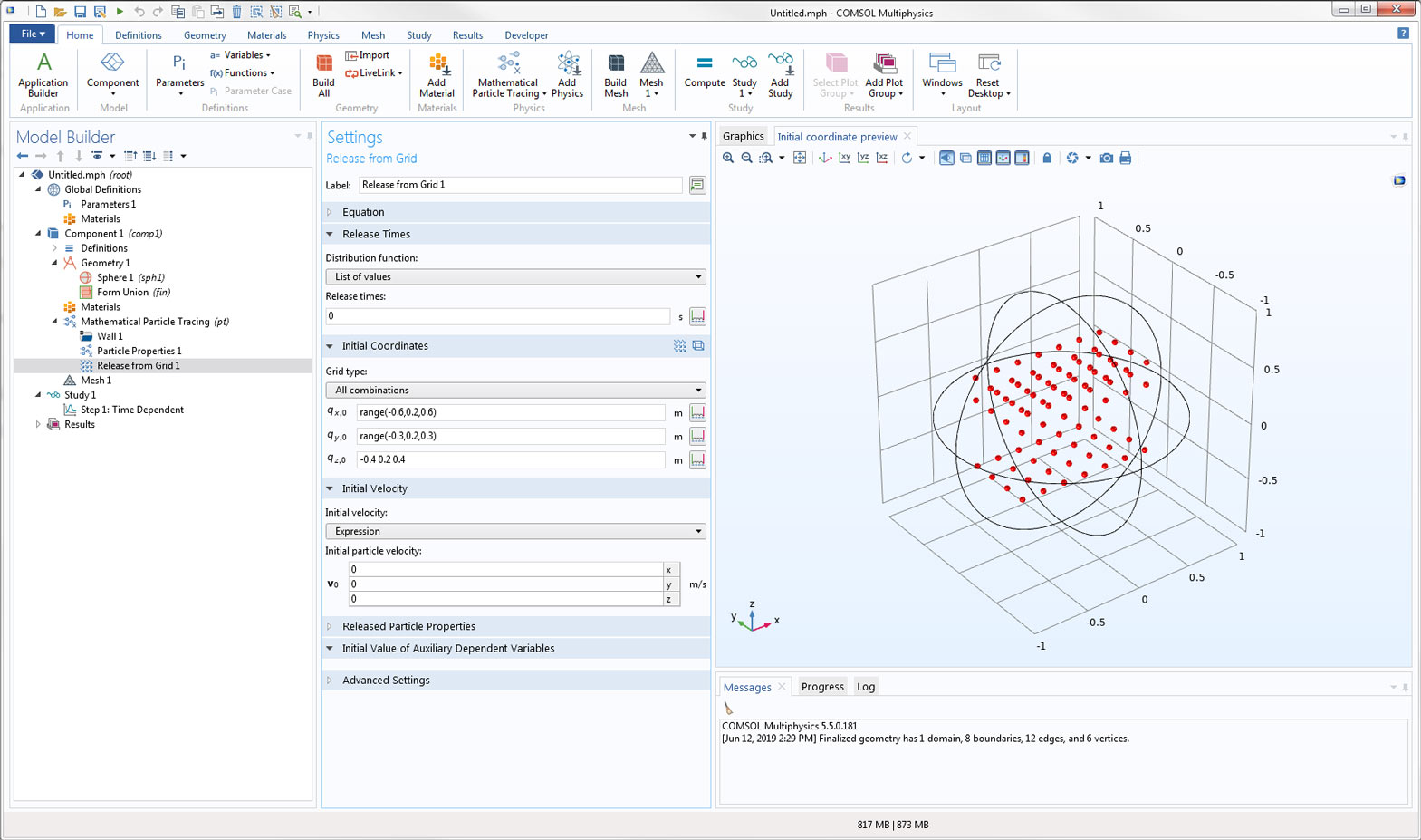
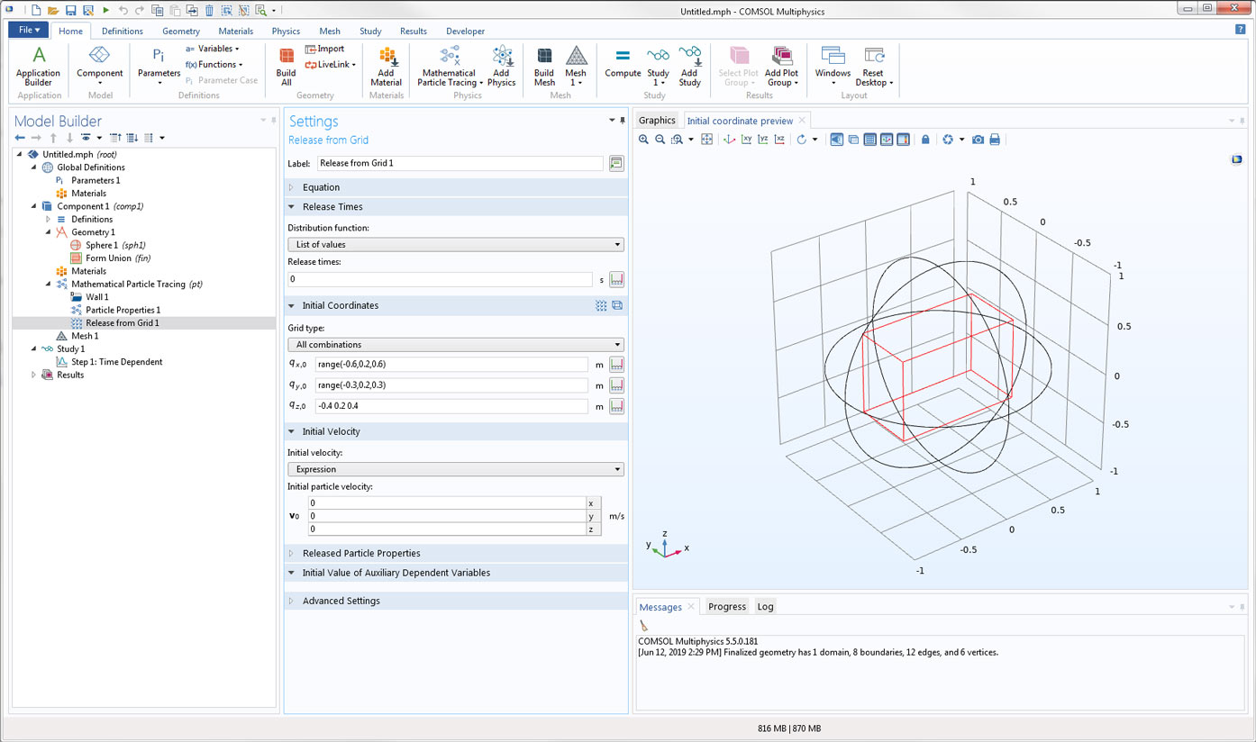
Preview Grid Release Positions
When you release particles from a grid of points using the Release from Grid feature, you can now preview the initial particle positions in the Graphics window. In the Initial Coordinates section of the Settings window, click the Preview Initial Coordinates button to view the initial particle coordinates as a grid of points. Click the Preview Initial Extents button to view the spatial extents of the initial coordinates as a bounding box. These buttons allow you to check the initial particle positions before running a study.
In addition, when you right-click a Study node and click Get Initial Value, you can preview the initial particle positions and velocities for all release types.
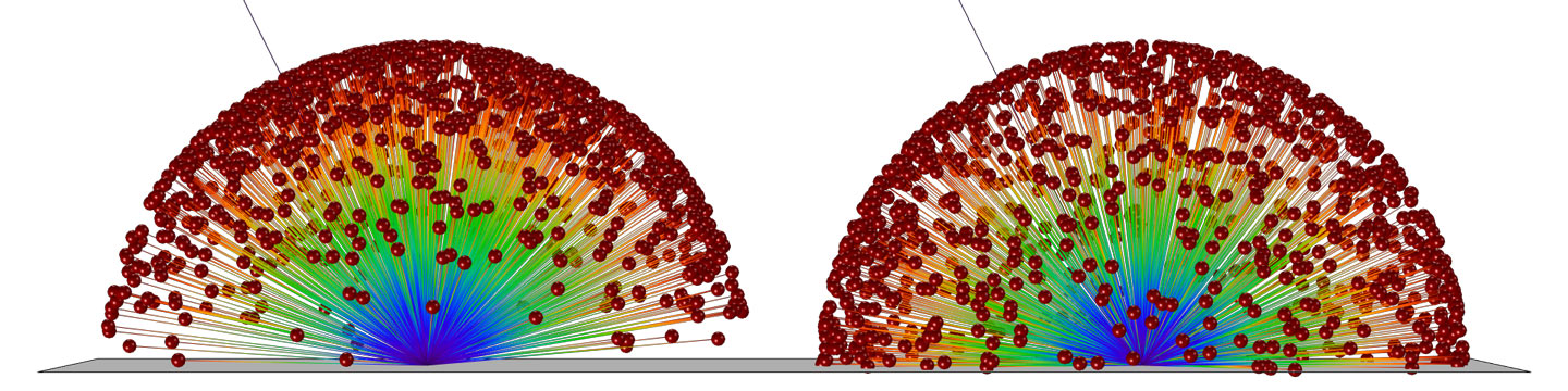
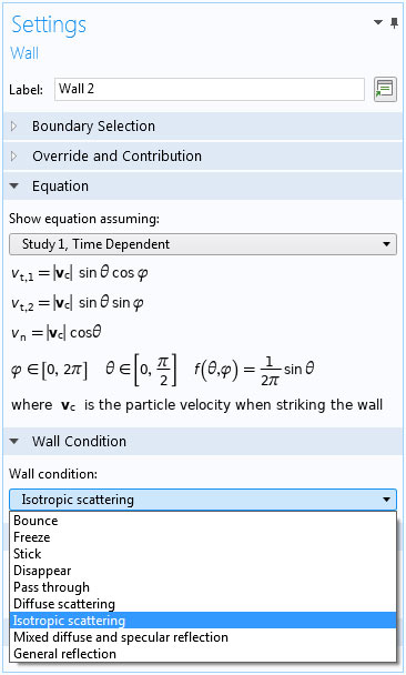
Isotropic Scattering Wall Condition
You can now select Isotropic scattering as the wall condition when particles hit boundaries in the geometry. Like the Diffuse scattering condition, the Isotropic scattering condition causes particles to be reflected with randomly sampled velocity directions around the surface normal. However, whereas the Diffuse scattering condition uses a probability distribution based on the cosine law, the Isotropic scattering condition follows a probability distribution that gives equal flux across any differential solid angle in the hemisphere.
New Tutorial Models and Applications
Version 5.5 brings several new tutorial models and applications.
Compact Camera Module
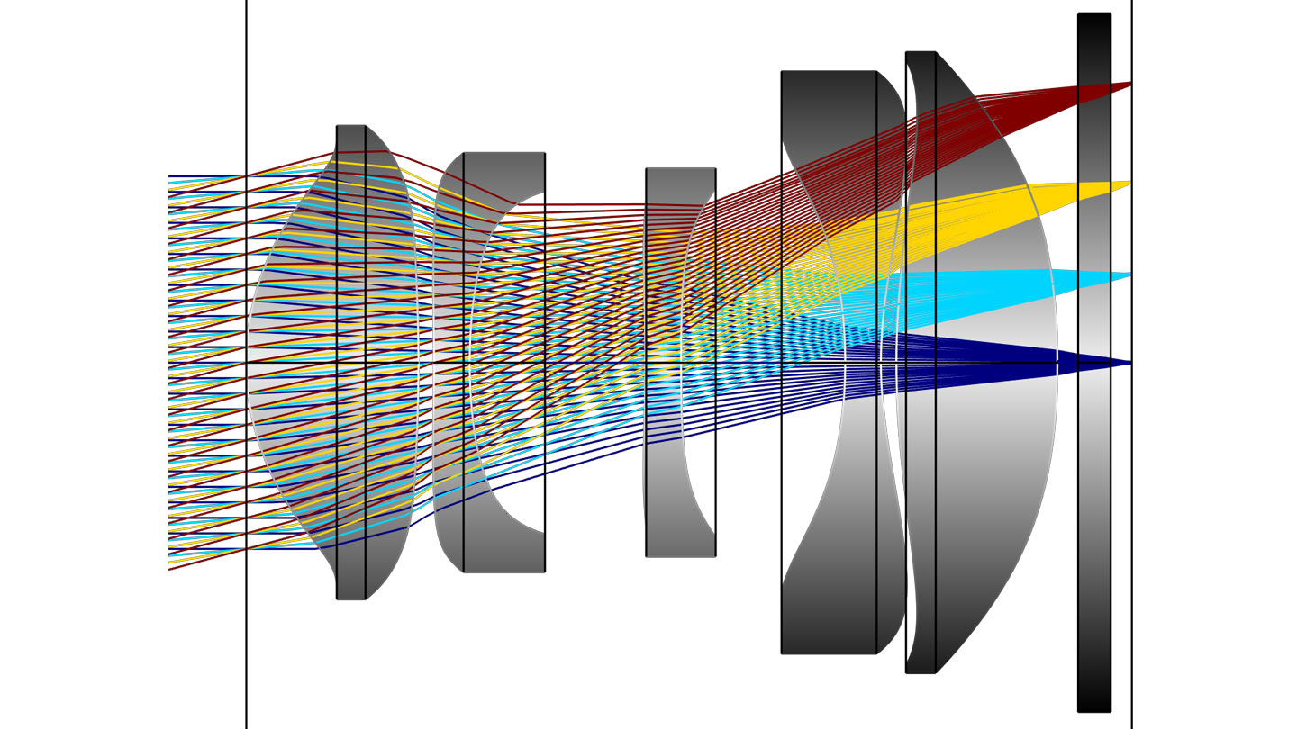
Application Library Title:
compact_camera_module
Gregory–Maksutov Telescope
Application Library Title:
gregory_maksutov_telescope
Keck Telescope
Application Library Title:
keck_telescope
Schmidt–Cassegrain Telescope
Application Library Title:
schmidt_cassegrain_telescope
Cross Grating Échelle Spectrograph
Application Library Title:
cross_grating_echelle_spectrograph
Newtonian Telescope Structural Analysis
Application Library Title:
newtonian_telescope_structural_analysis
Petzval Lens STOP Analysis with Hyperelasticity
Application Library Title:
petzval_lens_stop_analysis_with_hyperelasticity
Ray Release Based on a Plane Electromagnetic Wave
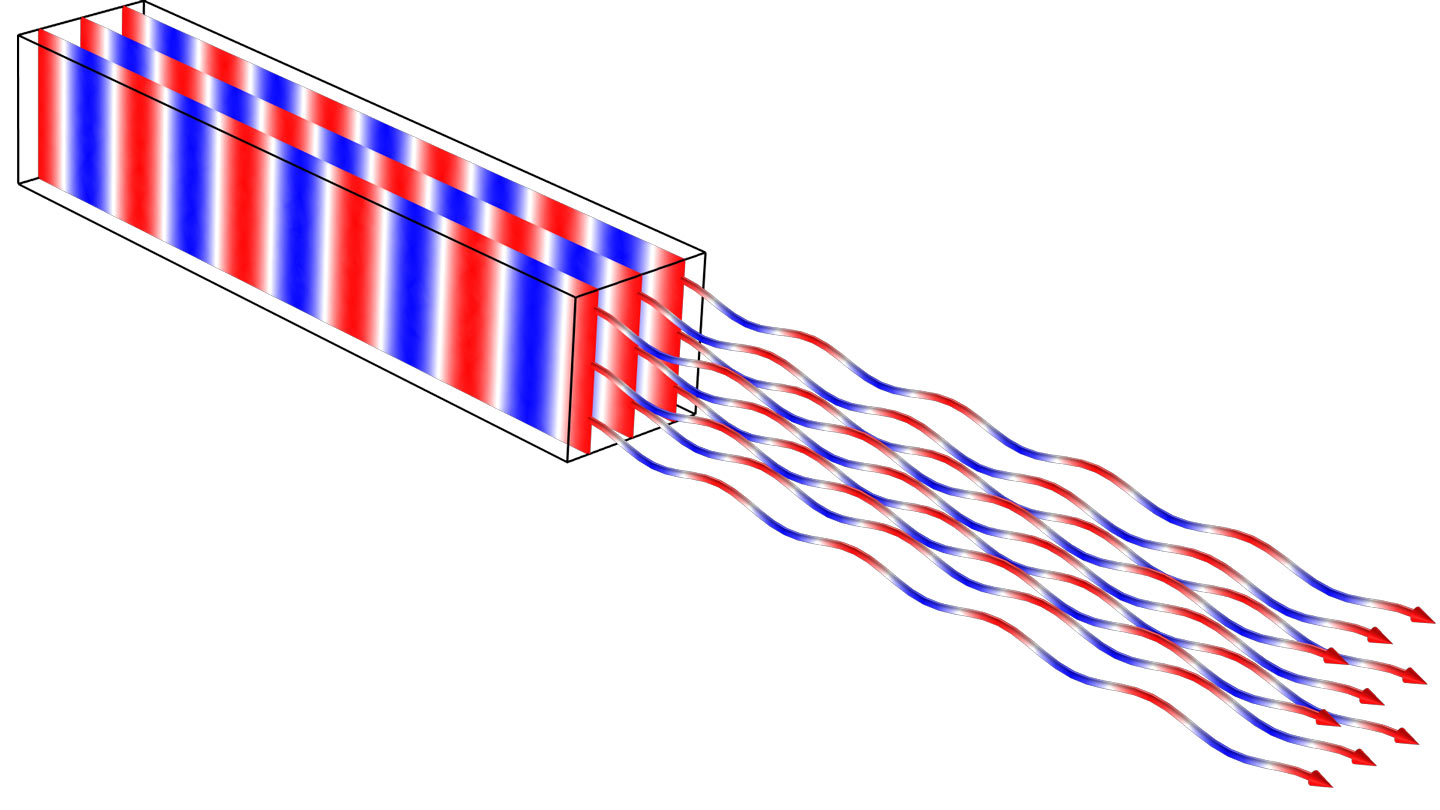
Application Library Title:
plane_em_wave_to_ray_release
Ray Optics with a Dipole Antenna Source (2D Axisymmetric)
Application Library Title:
ray_release_from_dipole_antenna_source_2daxi
Ray Optics with a Dipole Antenna Source (3D)
Application Library Title:
ray_release_from_dipole_antenna_source_3d