Neuerungen im Corrosion Module
Für Nutzer des Corrosion Module bietet COMSOL Multiphysics® Version 6.4 ein Interface zur Modellierung wässriger Elektrolyte, Variablen zur Bewertung von Energieverlusten sowie ein neues Feature zur Definition von Lade- und Entladezyklen. Weitere Informationen zu diesen und weiteren Updates finden Sie unten.
Neues Interface Aqueous Electrolyte Transport
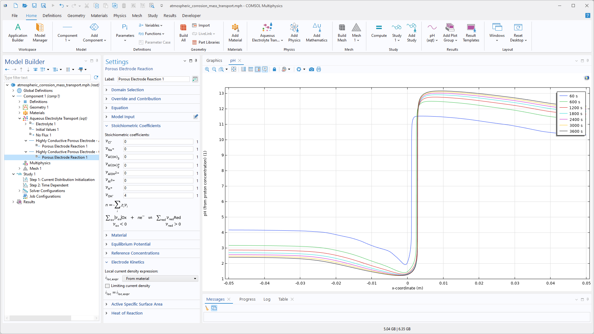
Für die Modellierung wässriger Elektrolyte mit schwachen Säuren, schwachen Basen, Ampholyten und generischen komplexen Spezies – sowie für Anwendungen wie mechanistische Korrosionsmodellierung, elektrochemische Modelle biologischer Systeme und elektrochemische Sensormodellierung – berechnet das neue Interface Aqueous Electrolyte Transport die Potential- und Spezieskonzentrationsfelder in einem verdünnten wässrigen Elektrolyten. Der Transport wird durch die Nernst-Planck-Gleichungen definiert, die Diffusion, Migration und Konvektion sowie Elektroneutralität und die Selbstionisationsgleichgewichtsreaktion von Wasser (Autoprotolyse) berücksichtigen. Aufgrund der effizienteren Handhabung von Gleichungsreaktionen und der einfacheren Modelleinrichtung ist das neue Interface in einigen Fällen möglicherweise dem allgemeineren Interface Tertiary Current Distribution, Nernst–Planck vorzuziehen.
Diese Funktionalität ist in den folgenden Tutorial-Modellen zu sehen:
- act_scratched_galvanized_steel
- atmospheric_corrosion_mass_transport
- crevice_corrosion_fe
- biodegradation_mg_stent
- evans_droplet
- co2_corrosion
Variablen zur Bewertung von Leistungsverlusten
Es ist nun möglich, den Betrag der Gesamtleistungsverluste in einer Batteriezelle zu bewerten und die Verluste zwischen einzelnen Komponenten wie Separator, Elektrode und Stromleiter zu vergleichen, indem neu eingeführte Leistungsverlustvariablen in den Electrochemistry -Interfaces verwendet werden. Diese Variablen können auch verwendet werden, um die Energieeffizienz einer Batteriezelle unter einem Lade-Entlade-Lastzyklus zu berechnen, indem die Leistungsverluste über die Zeit integriert werden.
Die Leistungsverluste werden auf der Grundlage der Verluste in der freien Gibbs-Energie aller reagierenden und transportierten Spezies definiert, wodurch zwischen ohmschen Verlusten, Konzentrationsverlusten und Aktivierungsverlusten unterschieden werden kann. In Batterien, die die Partikeleinlagerung unterstützen, werden auch separate Variablen für Einlagerungstransportverluste definiert. Diese Variablen sind lokal auf Gebieten und Rändern, als integrierte Werte über die gesamte Zelle oder pro einzelnem Modellbaumknoten verfügbar. Die Überspannungsbeiträge jedes Verlustmechanismus (ohmscher Verlust, Aktivierungsverlust und Transportverlust) können durch Division durch den Gesamtstrom berechnet werden.

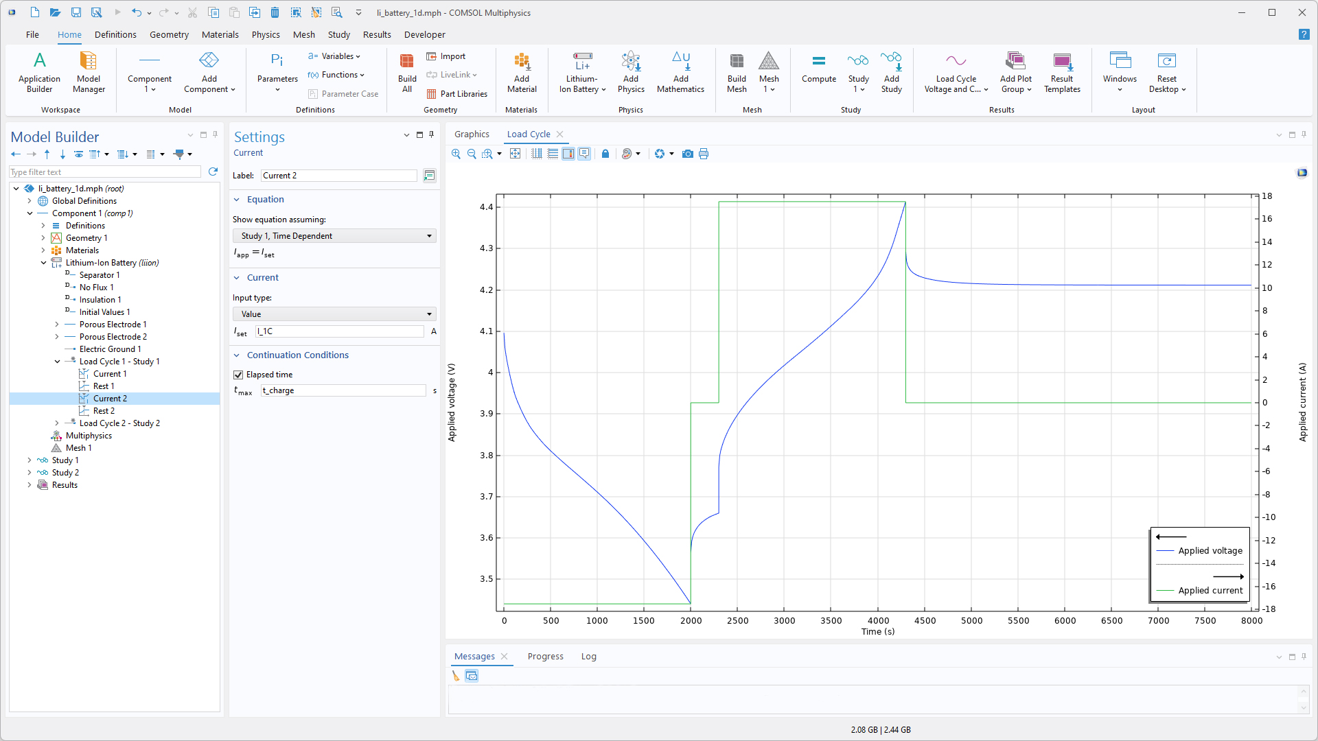
Neues Feature Load Cycle
Um das Aufsetzen komplexer Lastzyklen zu vereinfachen, wurde den meisten Electrochemistry-Interfaces ein neues Feature namens Load Cycle hinzugefügt. Mit diesem Feature lassen sich beliebige Lade-Entlade-Zyklen definieren, wobei die Schritte Voltage, Power, Current, C-rate und Rest in beliebiger Reihenfolge hinzugefügt werden können. Für jeden Schritt im Lastzyklus können ein oder mehrere dynamische Fortsetzungs- oder Unterbrechungskriterien (Umschaltkriterien) definiert werden, die auf Zeit-, Spannungs- oder Stromgrenzwerten sowie auf benutzerdefinierten Bedingungen unter Verwendung beliebiger Variablenausdrücke basieren können. Zusätzlich zu den vielseitigen Optionen zur Definition von Lastzyklen ermöglicht das neue Feature auch die automatische Definition von Strom- und Spannungssonden sowie von Löser-Stoppbedingungen.
Mit der Unterfunktion Subloop ist es beispielsweise möglich, Langzeit-Lade-Entlade-Zyklustests mit Referenzleistungstests zu kombinieren. Bitte beachten Sie, dass die Unterfunktionen Power und Subloop nur im Battery Design Module und im Fuel Cell & Electrolyzer Module verfügbar sind.
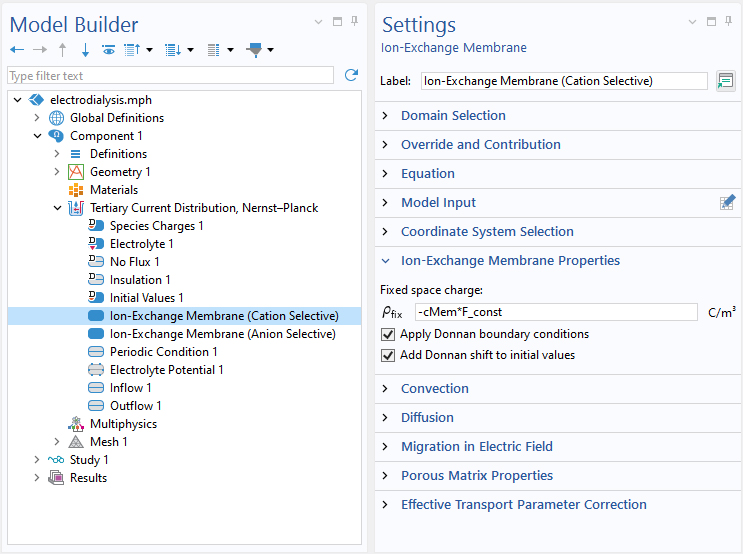
Automatische Initialisierung von Ionenaustauschmembranmodellen
Um Elektroneutralität und die Einhaltung des Donnan-Gleichgewichts sicherzustellen, enthält das Feature Ion-Exchange Membrane im Interface Tertiary Current Distribution, Nernst–Planck nun die Option Add Donnan shift to initial values. Diese Option verschiebt automatisch die im Feature Initial Values für den aktiven Gebietsknoten Ion-Exchange Membrane angegebenen Anfangskonzentrations- und Potenzialwerte, wobei davon ausgegangen wird, dass die benutzerdefinierten Werte die Werte für einen Flüssigelektrolyten im Gleichgewicht mit der Membran darstellen. Die verschobenen Anfangswerte werden dann als Anfangswerte für den Löser verwendet. Durch Aktivieren dieser Option wird die Modelleinrichtung in der Regel vereinfacht, da die feste Raumladung der Membran nicht mehr in einem zusätzlichen Studienschritt auf einen gewünschten Wert ungleich Null verschoben werden muss.
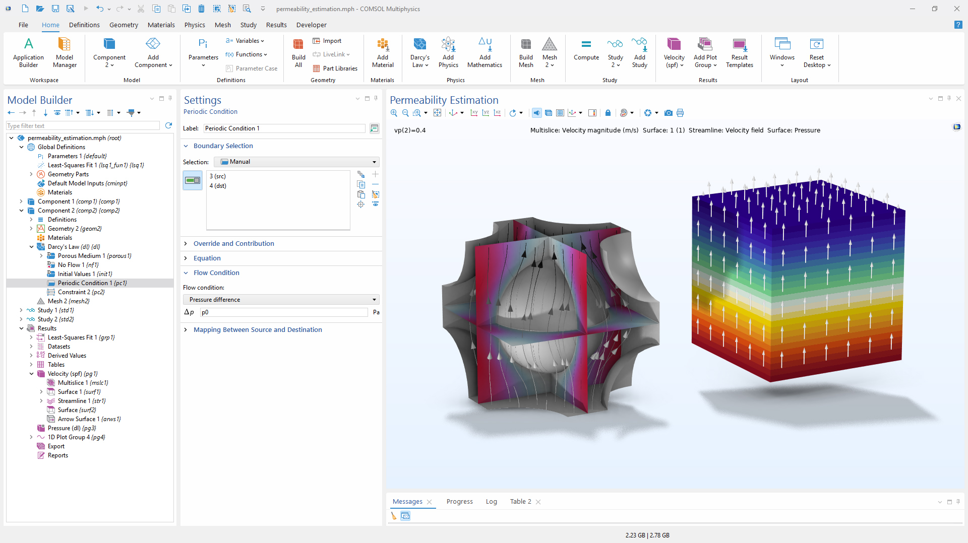
Periodic Condition
Die Interfaces Darcy's Law und Richards' Equation enthalten jetzt das neue Feature Periodic Condition, mit dem sich die Periodizität der Strömung zwischen zwei oder mehr Rändern festlegen lässt. Darüber hinaus ist es möglich, einen Druckunterschied zwischen Quell- und Zielrand zu erzeugen, indem entweder der Drucksprung direkt angegeben oder ein Massenstrom vorgegeben wird. Das Modell Estimating Permeability from Microscale Porous Structures veranschaulicht dieses neue Feature. Periodic Condition wird in der Regel verwendet, um repräsentative Volumenelemente zu modellieren und effektive Eigenschaften für die Verwendung in homogenisierten porösen Medien zu berechnen.
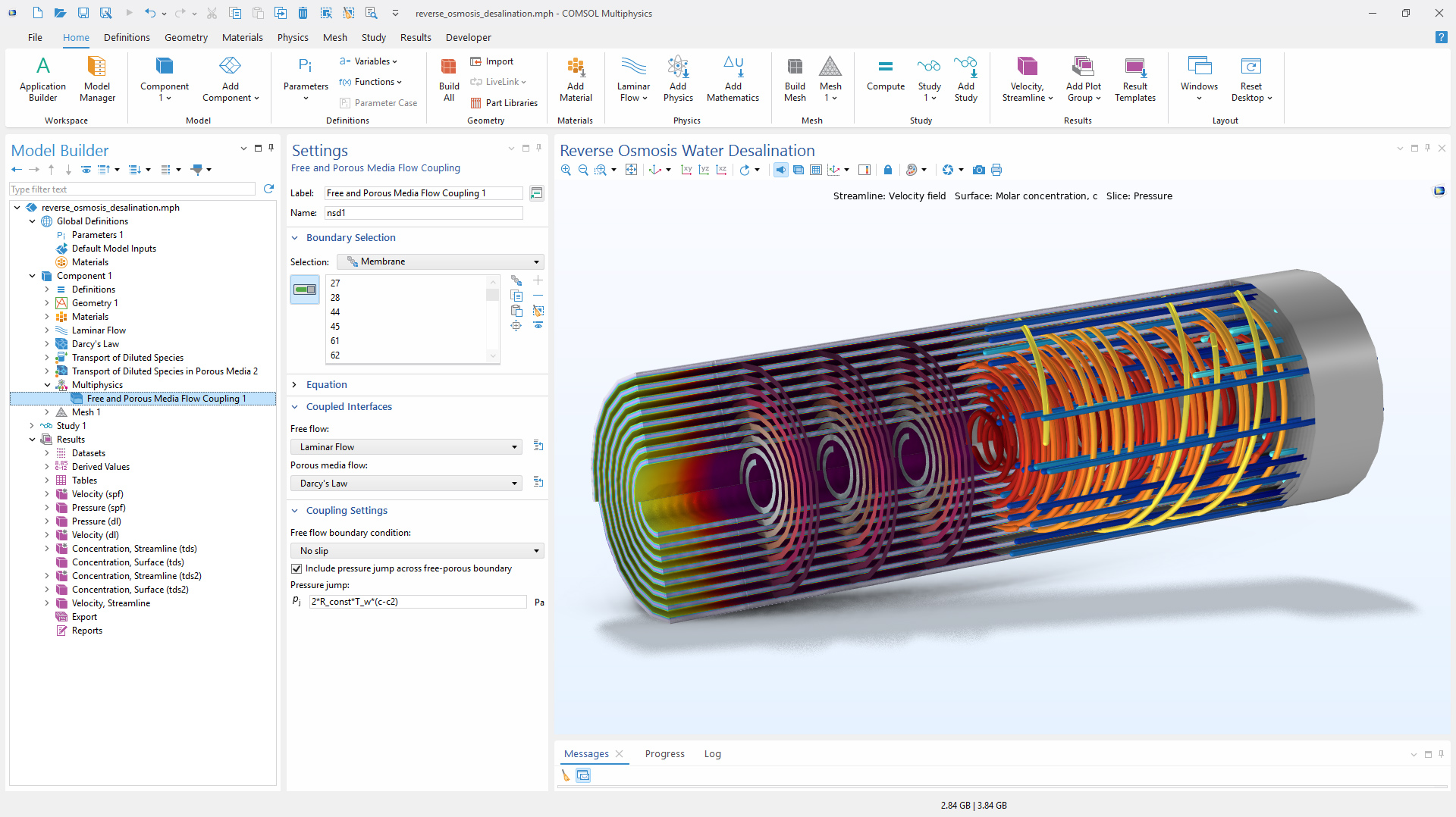
Drucksprungoption für Free and Porous Media Flow Coupling
Free and Porous Media Flow Coupling verfügt über eine neue Option, um einen Drucksprung über die Grenze zwischen freiem und porösem Medium hinweg einzubeziehen. Damit lassen sich beispielsweise der osmotische Druck an einer semipermeablen Membran, die von einem porösen Abstandsmaterial gestützt wird, oder ein Drucksprung aufgrund des Kapillardrucks bei einer Mehrphasenströmung modellieren.