Neuerungen im Bereich Ergebnisse und Visualisierung
COMSOL Multiphysics® Version 6.4 führt mehrere Verbesserungen für Ergebnisse und Visualisierung ein, darunter ausdrucksbasierte Transparenz, effizientere Erstellung von Plot-Arrays und verschiedene Verbesserungen für Stromlinien. Weitere Informationen zu diesen Updates und mehr finden Sie unten.
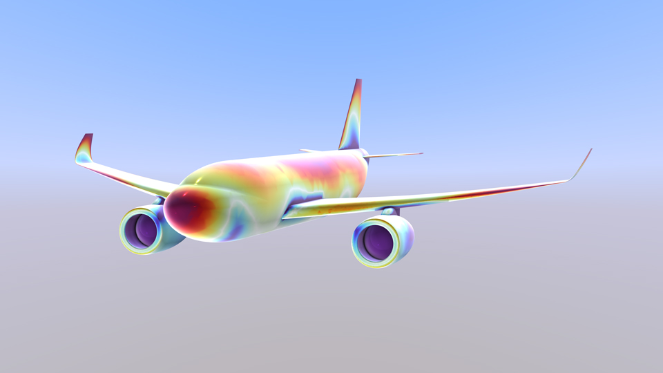
Ausdrucksdefinierte Transparenz
Das Subfeature Transparency kann nun verwendet werden, um die Transparenz mit einem Ausdruck zu definieren, ähnlich wie bei der Option Color Expression. Diese Funktion ermöglicht die Steuerung der Transparenz anhand von Modellgrößen, Parametern oder Funktionen und ermöglicht so erweiterte visuelle Effekte wie Überblenden, Schwellenwertbildung und multivariate Visualisierung. Beispielsweise ist es möglich, nach Temperatur zu färben und gleichzeitig die Transparenz nach Spannung oder Konzentration zu variieren, innere Bereiche ohne Schnitte sichtbar zu machen und realistischere transluzente Materialien zu erstellen. Die ausdrucksbasierte Transparenz funktioniert mit den meisten 3D-Plot-Typen sowie mit 2D-Plots, wenn Height Expression verwendet wird.
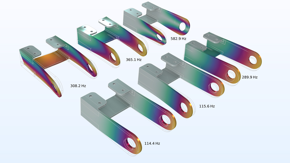
Solution Array
Das neue Subfeature Solution Array ermöglicht die nebeneinanderliegende Visualisierung mehrerer Lösungszustände, wie beispielsweise unterschiedliche Zeitpunkte, Eigenmoden oder Parameterwerte, innerhalb einer einzigen Plotgruppe. Es repliziert automatisch einen Plot für jeden ausgewählten Zustand, sodass Zeitverläufe, Modenformen oder Parametervariationen ohne erneutes Plotten leicht verglichen werden können. Die Anordnung und Gestaltung wird über alle Kacheln hinweg beibehalten, wodurch konsistente Farbskalen und Blickwinkel für visuell einheitliche und reproduzierbare Vergleiche gewährleistet sind.
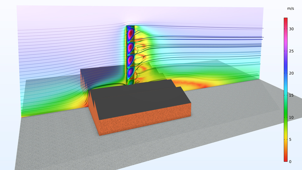
Verbesserungen der Stromlinien
Die betragsgesteuerte Punktverteilung kann nun für Stromlinien verwendet werden, die an ausgewählten Rändern beginnen. Dies kann dazu führen, dass mehr Stromlinien die qualitativ interessanten Teile der Strömung zeigen als bei Verwendung einer gleichmäßigen Punktverteilung. Darüber hinaus wurde die Runge-Kutta-Integration vierter Ordnung hinzugefügt, mit einer Option für adaptive Schrittlänge, was zu genaueren Stromlinien führen kann.
3D-Stromlinien werden nun so gerendert, dass sie eine Tiefenwahrnehmung vermitteln, was die Visualisierung verbessert, wenn viele Stromlinien dicht beieinander liegen. Die gleiche neue Rendering-Technik wird auch für Punkt- und Strahlbahnplots verwendet.

Verbesserungen der Environment Maps
Die Environment-Map-Funktionalität wurde flexibler gestaltet. Diese erweiterte Funktionalität kann zur Verbesserung der Visualisierung glänzender Materialien und als Hintergrund für Plots oder Geometrien verwendet werden. Zu den wichtigsten Neuerungen gehören:
- Unterstützung für Sky–Ground Maps, die durch vier Farben definiert sind: zwei für den Himmel und zwei für den Boden
- Unterstützung für benutzerdefinierte Maps, die aus einem gleichwinkligen Bild oder einer Cube Map erstellt wurden
- Es wurden fünf neue vordefinierte Environment Maps hinzugefügt: vier auf Bildern basierende und eine Sky–Ground Map