Neuerungen im Battery Design Module
Für Nutzer des Battery Design Module bietet COMSOL Multiphysics® Version 6.4 neue Variablen für Leistungsverluste, die Möglichkeit, beliebige Lade- und Entladezyklen zu definieren, sowie eine deutlich benutzerfreundlichere und genauere Modellierung des Wärmetransports in prismatischen Batterien. Weitere Informationen zu diesen und weiteren Updates finden Sie unten.
Variablen zur Bewertung von Leistungsverlusten
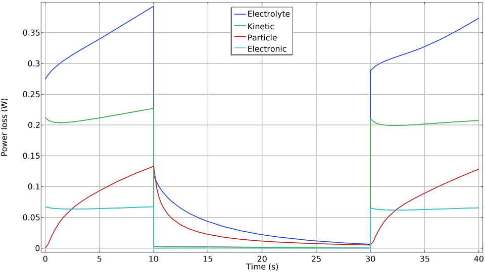
Es ist nun möglich, den Betrag der Gesamtleistungsverluste in einer Batteriezelle zu bewerten und die Verluste zwischen einzelnen Komponenten wie Separator, Elektrode und Stromleiter zu vergleichen, indem neu eingeführte Leistungsverlustvariablen in den Electrochemistry Interfaces verwendet werden. Diese Variablen können auch verwendet werden, um den Round-Trip-Wirkungsgrad einer Batteriezelle unter einem Lade-Entlade-Zyklus zu berechnen, indem die Leistungsverluste über die Zeit integriert werden.
Die Leistungsverluste werden auf der Grundlage der Verluste in der freien Gibbs-Energie aller reagierenden und transportierten Spezies definiert, wodurch zwischen ohmschen Verlusten, Konzentrationsverlusten und Aktivierungsverlusten unterschieden werden kann. In Batterien, die Partikelinterkalation unterstützen, werden auch separate Variablen für Interkalationstransportverluste definiert. Diese Variablen sind lokal auf Gebieten und Rändern, als integrierte Werte über die gesamte Zelle oder pro einzelnem Modellbaumknoten verfügbar. Die Überspannungsbeiträge jedes Verlustmechanismus (ohmscher Verlust, Aktivierungsverlust und Transportverlust) können durch Division durch den Gesamtstrom berechnet werden.
Diese Funktionalität ist in dem neuen Tutorial-Modell Power Losses in a Lithium-Ion Battery zu sehen.

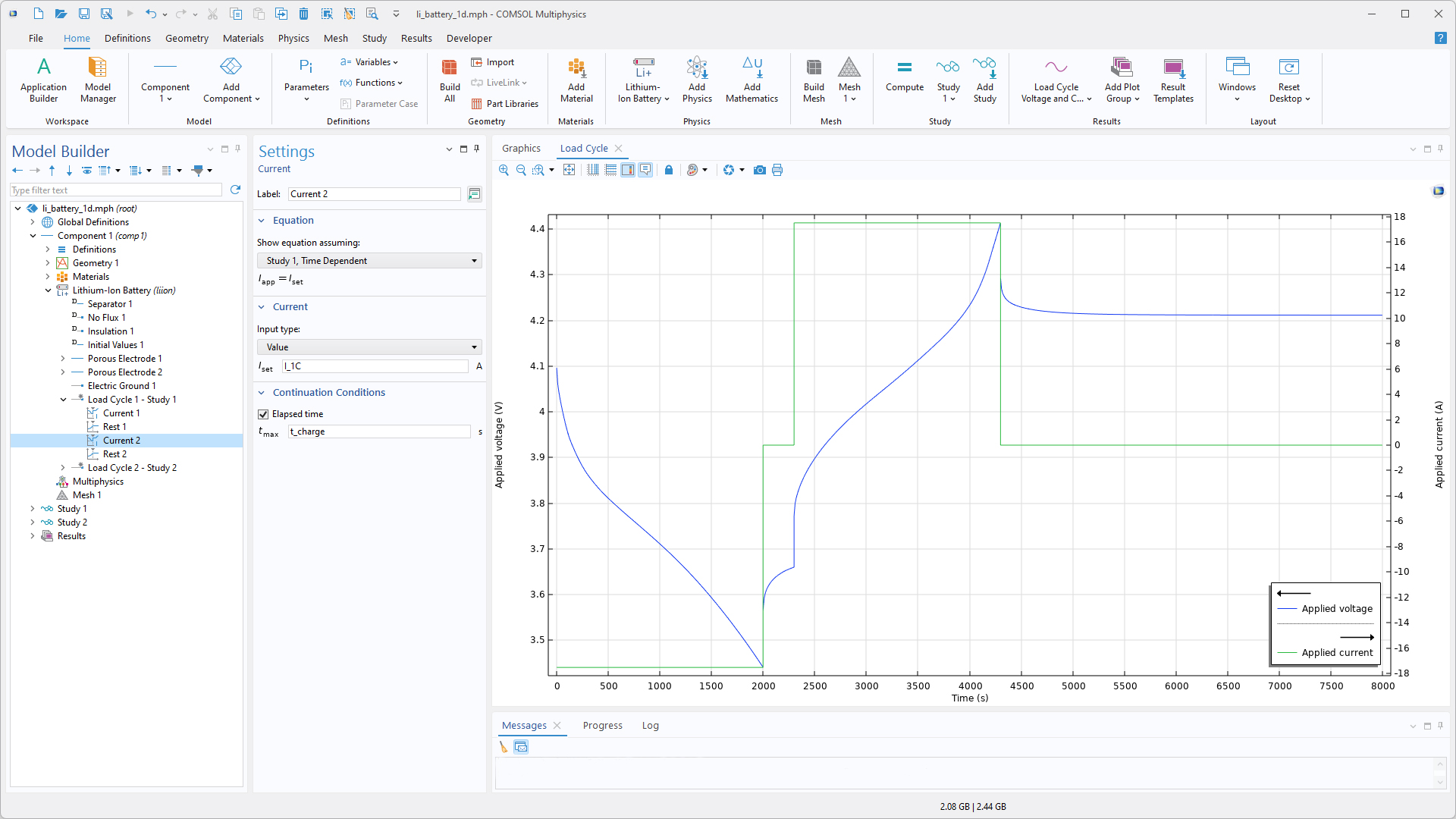
Neues Feature Load Cycle
Um die Einrichtung komplexer Zyklusprogramme zu vereinfachen, wurde den meisten Electrochemistry Interfaces ein neues Feature namens Load Cycle hinzugefügt. Mit diesem Feature können beliebige Lade- und Entladezyklen definiert werden, wobei die Schritte Voltage, Power, Current, C-rate und Rest in beliebiger Reihenfolge hinzugefügt werden können. Für jeden Schritt im Lastzyklus können ein oder mehrere dynamische Fortsetzungs- oder Unterbrechungskriterien (Umschaltkriterien) definiert werden, die auf Zeit-, Spannungs- oder Stromgrenzwerten sowie auf benutzerdefinierten Bedingungen unter Verwendung beliebiger variabler Ausdrücke basieren können. Zusätzlich zu den vielseitigen Optionen zur Definition von Lastzyklen ermöglicht das neue Feature auch die automatische Definition von Strom- und Spannungssonden sowie von Stoppbedingungen für den Löser.
Mit der Unterfunktion Subloop ist es beispielsweise möglich, Langzeit-Lade-Entlade-Zyklustests mit Referenzleistungstests zu kombinieren. Die Unterfunktionen Power und Subloop sind nur im Battery Design Module und im Fuel Cell & Electrolyzer Module verfügbar.
Die folgenden Tutorial-Modelle wurden aktualisiert, um dieses Feature zu veranschaulichen:
- li_battery_1d
- lib_base_model_1d
- lib_diffusion_induced_stress
- li_rate_capability
- lib_drive_cycle
- lib_single_particle
- li_battery_multiple_materials_1d
- li_plating_with_deformation
- zn_ago_battery_1d
- lithium_sulfur
- li_battery_thermal_2d_axi
- li_battery_thermal_3d
- li_battery_pack_3d
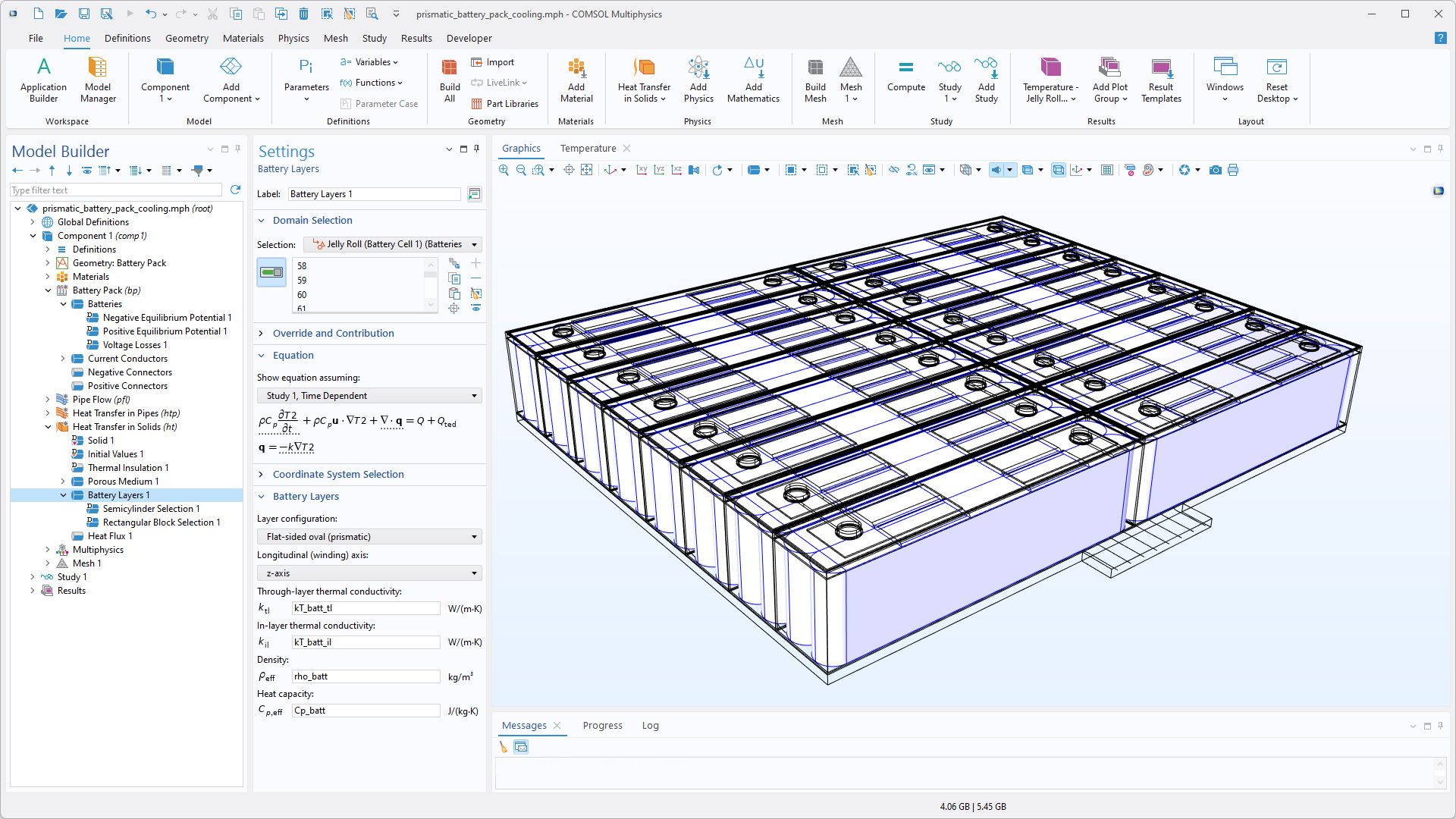
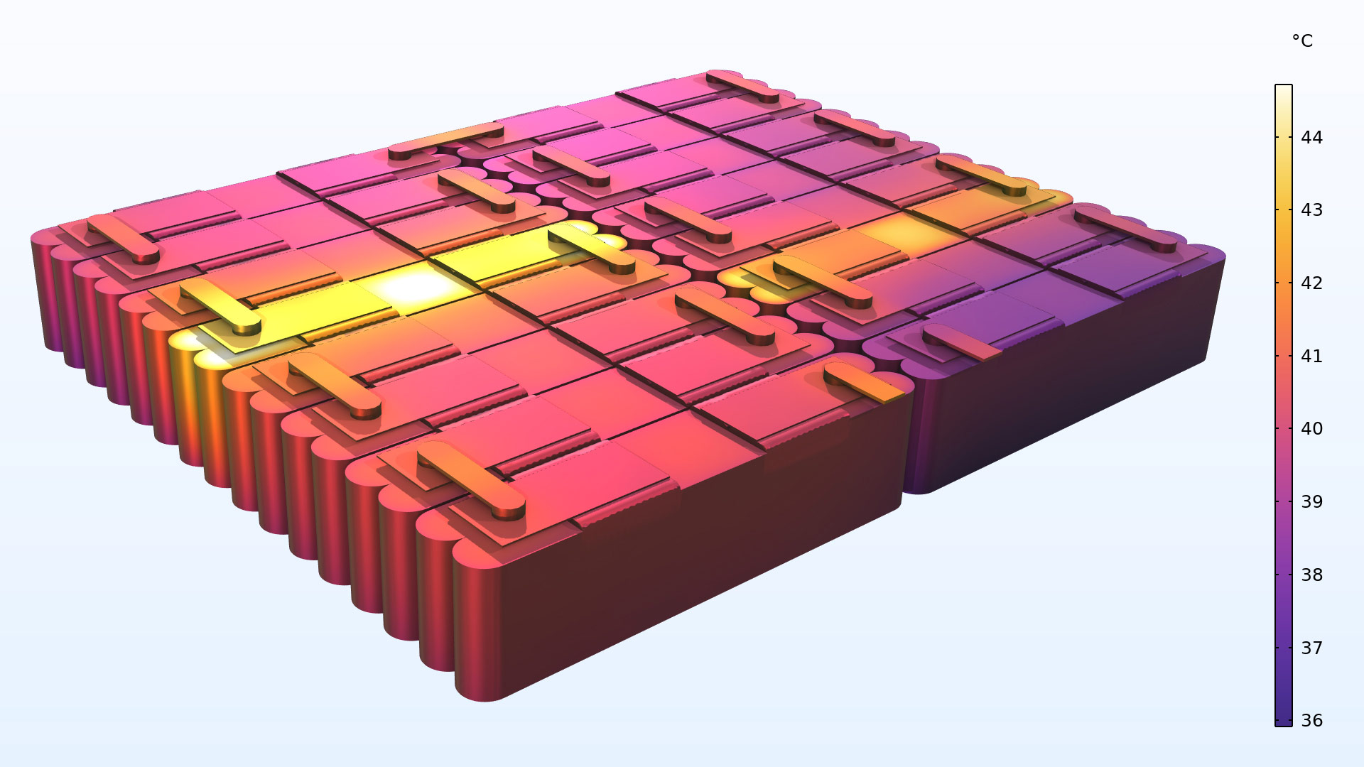
Wärmetransport in prismatischen Batterien
Um eine genaue Modellierung des Wärmetransports in prismatischen Batterien zu ermöglichen, wurde dem Knoten Battery Layers in den Heat Transfer Interfaces eine neue Option für die Schichtkonfiguration namens Flat-sided oval (prismatic) hinzugefügt.
Mit den Unterfunktionen Semicylinder Selection und Rectangular Block Selection kann das Feature Battery Layers nun automatisch die kombinierten zylindrischen und kartesischen Koordinatensysteme definieren, die zur korrekten Angabe anisotroper Wärmeleitfähigkeitstensoren in prismatischen Jelly Rolls erforderlich sind. Dies ermöglicht eine genaue Beschreibung der Wärmeleitfähigkeit in der Jelly Roll unter Berücksichtigung der verschiedenen Batteriekomponentenschichten und ihrer Wicklung. Sehen Sie sich diese neue Funktionalität in den Tutorial-Modellen Liquid-Cooled Prismatic Battery Pack und Cooling of a Prismatic Battery an.
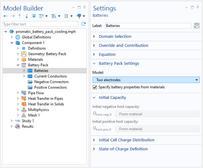
Modelloption Two Electrodes im Interface Battery Pack
Um das Verhalten einzelner Elektroden in jeder Batteriezelle eines Batteriepacks zu modellieren, steht die Modelloption Two electrodes, die zuvor im Interface Lumped Battery verfügbar war, nun auch im Interface Battery Pack zur Verfügung.
Mit dieser Modelloption können das Elektrodenpotenzial, die anfängliche Wirtskapazität und der Umwandlungsgrad für die beiden Elektroden in jeder Zelle separat definiert werden. Außerdem können damit individuelle Elektrodeneigenschaften definiert werden, um ohmsche, Aktivierungs- und Konzentrationsüberspannungen zu berücksichtigen. Wenn Konzentrationsüberspannungen einbezogen werden, entspricht das Modell Two electrodes dem, was in der Literatur gemeinhin als Einzelpartikelmodell (single-particle model, SPM) bezeichnet wird. Diese Funktionalität können Sie sich in dem neuen Tutorial-Modell Liquid-Cooled Prismatic Battery Pack ansehen.
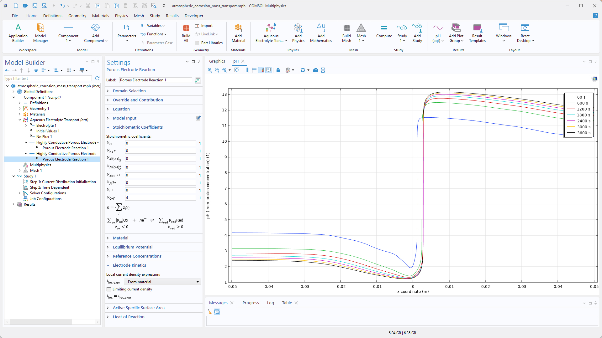
Neues Interface Aqueous Electrolyte Transport
Für die Modellierung wässriger Elektrolyte mit schwachen Säuren, schwachen Basen, Ampholyten und generischen komplexen Spezies – sowie für Anwendungen wie mechanistische Korrosionsmodellierung, elektrochemische Modelle biologischer Systeme und elektrochemische Sensormodellierung – berechnet das neue Interface Aqueous Electrolyte Transport die Potential- und Spezieskonzentrationsfelder in einem verdünnten wässrigen Elektrolyten. Der Transport wird durch die Nernst-Planck-Gleichungen definiert, die Diffusion, Migration und Konvektion sowie Elektroneutralität und die Gleichgewichtsreaktion für die Selbstionisation von Wasser (Autoprotolyse) berücksichtigen. Aufgrund der effizienteren Handhabung von Gleichgewichtsreaktion und der einfacheren Modelleinrichtung ist das neue Interface in einigen Fällen möglicherweise gegenüber dem allgemeineren Interface Tertiary Current Distribution, Nernst–Planck vorzuziehen.
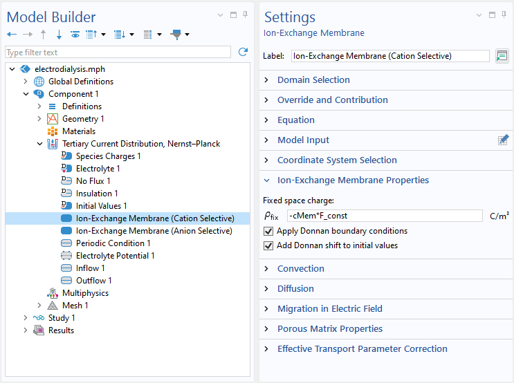
Automatische Initialisierung von Ionenaustauschmembranmodellen
Um Elektroneutralität und die Einhaltung des Donnan-Gleichgewichts sicherzustellen, enthält das Feature Ion-Exchange Membrane im Interface Tertiary Current Distribution, Nernst–Planck nun die Option Add Donnan shift to initial values. Diese Option verschiebt automatisch die im Feature Initial Values für den aktiven Gebietsknoten Ion-Exchange Membrane angegebenen Anfangskonzentrations- und Potenzialwerte. Dabei wird davon ausgegangen, dass die benutzerdefinierten Werte die Werte für einen Flüssigelektrolyten im Gleichgewicht mit der Membran darstellen. Die verschobenen Anfangswerte werden dann als Anfangswerte für den Löser verwendet. Durch Aktivieren dieser Option wird die Modellerstellung in der Regel vereinfacht, da die feste Raumladung der Membran nicht mehr in einem zusätzlichen Studienschritt auf einen gewünschten Wert ungleich Null verschoben werden muss. Diese Funktion können Sie sich im Tutorial-Modell Vanadium Redox Flow Battery ansehen.
Periodic Condition
Die Interfaces Darcy's Law und Richards' Equation enthalten jetzt das neue Feature Periodic Condition, mit dem sich die Periodizität der Strömung zwischen zwei oder mehr Rändern festlegen lässt. Darüber hinaus ist es möglich, einen Druckunterschied zwischen Quell- und Zielrand zu erzeugen, indem entweder der Drucksprung direkt angegeben oder ein Massenstrom vorgegeben wird. Periodic Condition wird in der Regel verwendet, um repräsentative Volumenelemente zu modellieren und effektive Eigenschaften für die Verwendung in homogenisierten porösen Medien zu berechnen.

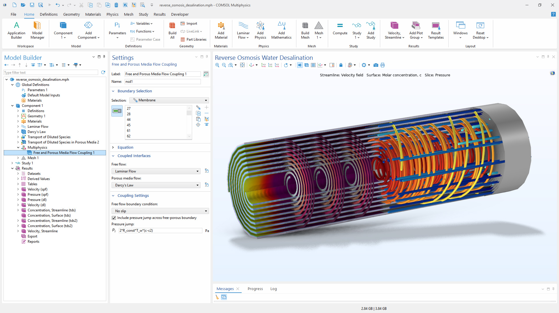
Drucksprungoption für Free and Porous Media Flow Coupling
Free and Porous Media Flow Coupling verfügt über eine neue Option, um einen Drucksprung über den Rand zwischen freiem und porösem Medium hinweg einzubeziehen. Damit lassen sich beispielsweise der osmotische Druck an einer semipermeablen Membran, die von einem porösen Abstandsmaterial gestützt wird, oder ein Drucksprung aufgrund des Kapillardrucks bei einer Mehrphasenströmung modellieren.
Neue und aktualisierte Tutorial-Modelle
COMSOL Multiphysics® Version 6.4 enthält mehrere neue und aktualisierte Tutorial-Modelle für das Battery Design Module.
Liquid-Cooled Prismatic Battery Pack
Open-Circuit Voltage and Differential Voltage Modeling of a Lithium-Ion Battery

Voltage Hysteresis in a Lithium Iron Phosphate (LFP) Electrode

Minimizing the Charging Time of a Lithium-Ion Battery
Power Losses in a Lithium-Ion Battery